Lecture 04 · 29 slides · August 17, 2026

Positional Encoding — telling attention where things live.

Raw self-attention has no built-in notion of order. Without positional information, it cannot distinguish the dog bit the man from the man bit the dog. This lecture compares several ways to give transformers a sense of position, including the case for learning without an explicit encoding.

Lecture 04 29 slides Manish Shrivastava · Aparajitha

§0The deck at a glance

The deck first explains why order matters, then compares absolute, sinusoidal, relative, and RoPE encodings in terms of their strengths and limitations. It ends with NoPE, the finding that a causal decoder can sometimes infer position from its attention mask.

§1Why position matters

Before we pick an encoding, we have to be clear about what is broken. Self-attention takes a set of vectors and returns a set of vectors — every query looks at every key by dot-product similarity, and the similarity does not know or care where in the sequence either token came from. Language, unlike a bag of marbles, has order. Three slides set that up.

Slide 01 / 29

Title slide: Positional Embedding, Advanced NLP M26, Manish Shrivastava and Aparajitha, August 17 2026, IIIT Hyderabad

slide 01 · title

On the slide

Title card for Lecture 4 of Advanced NLP, Monsoon '26. Delivered by Manish Shrivastava and Aparajitha on August 17, 2026.

What to take from it

The title says positional embedding rather than "positional encoding". In this course we use the two terms interchangeably. Strictly, an embedding is a learned vector table, and an encoding is a fixed function — but modern usage smears them together, and so will we.

Slide 02 / 29

Vaswani transformer architecture diagram with the Positional Encoding block on the encoder input circled in red

slide 02 · where positional encoding lives

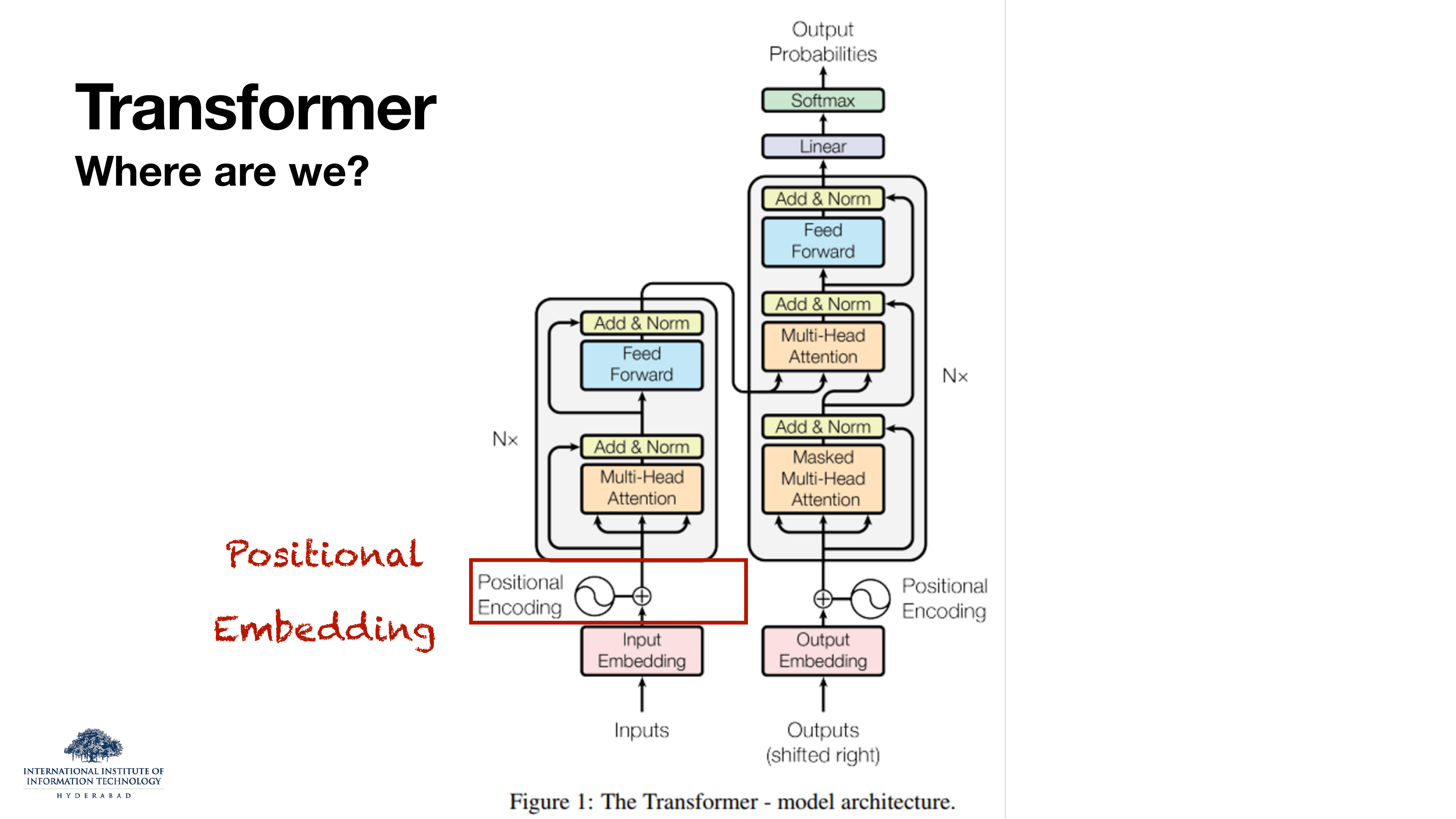
On the slide

The original Vaswani et al. (2017) transformer diagram. The lecturer has drawn a red box around the positional encoding block sitting under the input embedding, on both encoder and decoder sides. That is the whole real estate this lecture is about.

What to take from it

Read the diagram from the bottom up. Words become input embeddings — vectors of size d_model. Those vectors are then summed with a positional encoding vector of the same size. Only that sum enters the first attention layer. So position enters the network exactly once, at the very bottom, as an additive offset to the token embedding — and every layer above has to route that information wherever it needs it.

✦ Key takeaway

Attention is permutation-equivariant: shuffle the input rows and the output rows shuffle the same way. So without something like this red box, the model would give the dog bit the man and man the bit dog the identical hidden states. Everything in this lecture is a different answer to "what should go in that red box?"

Slide 03 / 29

Word Position — Importance. Bullets: Languages have order of the sequence (no free order, relative free order); Noun/Verb modifiers; Causality; Temporal

slide 03 · why order carries meaning

On the slide

Five reasons position is not a nuisance detail but a first-class linguistic signal.

Order of the sequence. Some languages are no-free-order (English: the dog bit the man ≠ the man bit the dog). Others are relative-free-order (Hindi, Sanskrit, Latin), where words can move around but the relative positions of a noun and its modifier still matter.
Noun/Verb modifiers. An adjective attaches to the noun next to it; an adverb attaches to the verb next to it. Which noun or verb "next to it" means is a positional question.
Causality. The glass broke because he dropped it — the "because" clause only makes sense as the reason if it comes after the effect. Swap them and the causal reading flips.
Temporal. Narratives ("first she opened the door, then she left") encode time via order.

⚠ Watch out

"Hindi has free word order, so position doesn't matter there" is a myth. Hindi is relatively free — the argument order in राम ने सीता को देखा vs. सीता को राम ने देखा can move, but the case markers and the modifier-head adjacency are still position-carried. Any transformer used for Hindi still needs positional encoding.

§2Absolute PE — the naive first try

The most straightforward answer: give every position a vector, look it up like you look up a word, add it to the token embedding. This is how BERT and GPT-2 do it, and it works — with two nagging problems the deck will make you feel.

Slide 04 / 29

slide 04 · section divider

A section divider. The next two slides describe absolute positional embedding — one vector per position, learned like an ordinary embedding table.

Slide 05 / 29

Absolute PE Approach: vectors with the same dimension as the word itself; each word gets a unique absolute embedding to show its position in the sentence

slide 05 · approach

Slide 06 / 29

Absolute PE Drawbacks: model just remembers the position vectors; no information about relative positions; struggle to predict unseen (during training) positions

slide 06 · drawbacks

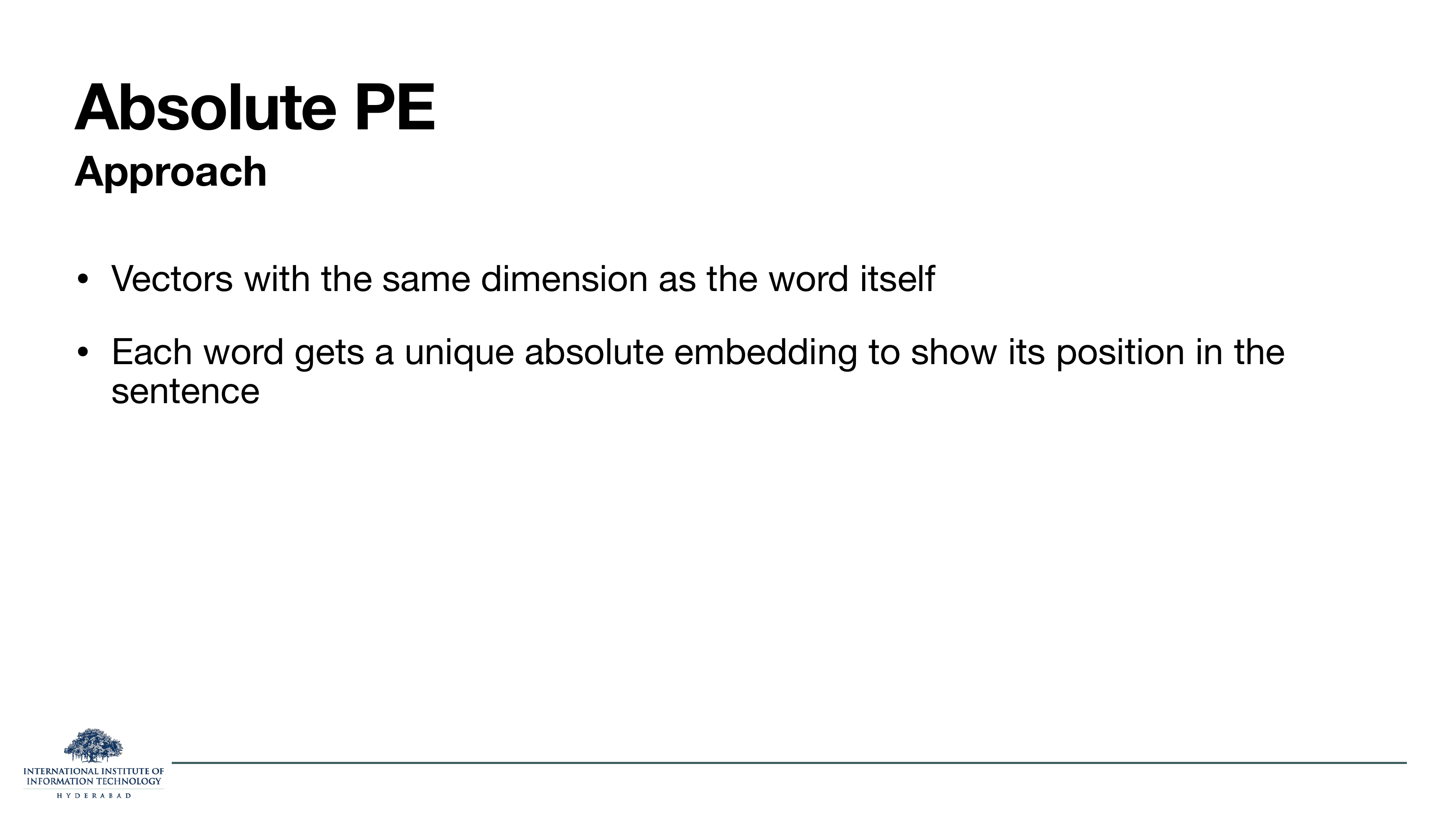
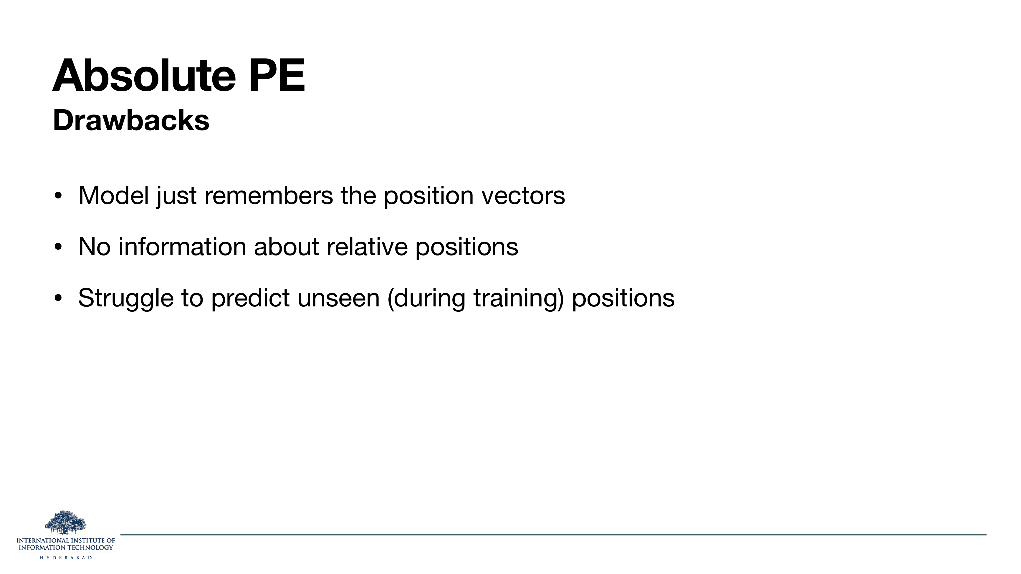
What these two slides show

Slide 5 is the recipe: an absolute PE is a vector of the same dimension as the word embedding — call it d_model — and each position pos = 0, 1, 2, …, L−1 gets one such vector. During training these vectors are stored in a lookup table and learned by gradient descent, exactly like the word embedding table. The position vector is added to the word vector before the first attention layer.

Slide 6 is the honest post-mortem: three concrete failure modes.

h_{i} = WordEmb (w_{i}) + PosEmb (i)

Why the drawbacks hurt

"Model just remembers the position vectors." Every position is an independent parameter. Position 42 and position 43 have no reason to be similar to each other — the model has to learn from data that adjacent positions should behave similarly, and it usually does, but nothing in the parameterisation forces it.
No relative-position information. The attention score between token at position 5 and token at position 12 has no built-in notion of "they are 7 apart". The model has to reconstruct that distance from the difference of two absolute lookups, which is hard.
Cannot extrapolate. If you trained with a maximum sequence length of 512, position 513 has no vector — the lookup table simply doesn't have that row. At test time you either have to truncate or reinitialise, and both hurt.

⚠ Watch out

BERT was trained with max length 512 exactly because of this. That's not an accident of engineering — it is a direct consequence of using absolute embeddings.

§3Sinusoidal PE — the Vaswani recipe

The original transformer paper picked a different design: instead of learning the position table, compute it from a fixed formula built out of sines and cosines at exponentially spaced frequencies. Five slides justify why that fixed formula was chosen and where it still falls short.

Slide 07 / 29

slide 07 · section divider

Section header. The next four slides walk through the sinusoidal encoding used in Attention is All You Need.

Slide 08 / 29

$Sinusoidal PE Approach. Hypothesis: allow the model to easily learn to attend by relative positions. For any fixed offset k, PE_{pos+k} can be represented as a linear function of PE_{pos}. Added to the word embedding. Cites Vaswani et al 2017.$

slide 08 · approach and hypothesis

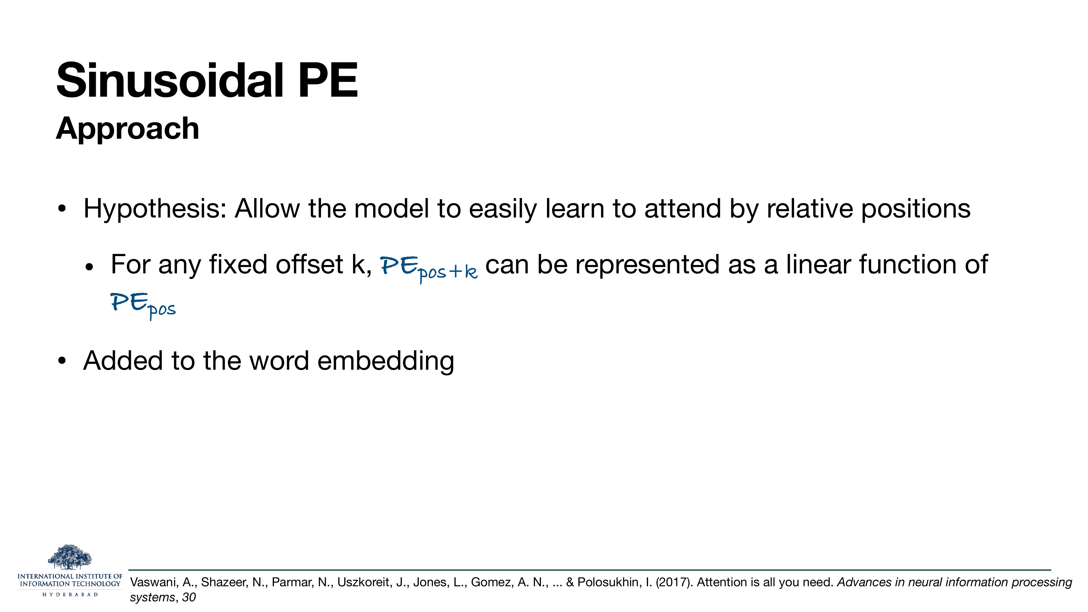
On the slide

Vaswani et al.'s design hypothesis, in one line: choose a positional encoding function such that the encoding at position pos+k is a linear function of the encoding at position pos, for any fixed offset k.

Why that specific property

Self-attention computes a dot product of query and key. If two positions differ by a fixed amount k, the model should be able to compute their attention score in a way that only depends on k, not on where in the sentence they happen to sit. A linear-shift-invariant encoding gives you exactly that: the model can learn a linear head that fires whenever two tokens are, say, 3 apart, regardless of whether they are at positions (0, 3) or (100, 103).

Sines and cosines have this property for free — this is essentially the rotation identity $\sin (a + b) = \sin a \cos b + \cos a \sin b$ , which is a linear combination of sin(a) and cos(a) with coefficients depending only on the shift b.

→ Keep reading

This same "relative-shift is a linear map" idea gets recycled in RoPE (§5), except there the linear map is a genuine rotation matrix acting on the query/key vectors themselves.

Slide 09 / 29

$Sinusoidal PE formula: PE_{(pos, 2i)} = sin(pos / 10000^{2i/d_model}) and PE_{(pos, 2i+1)} = cos(pos / 10000^{2i/d_model}). Below: coloured bars showing positional encoding vectors summed with x1, x2, x3 embeddings for the French words Je, suis, étudiant.$

slide 09 · the formula, in one picture

On the slide

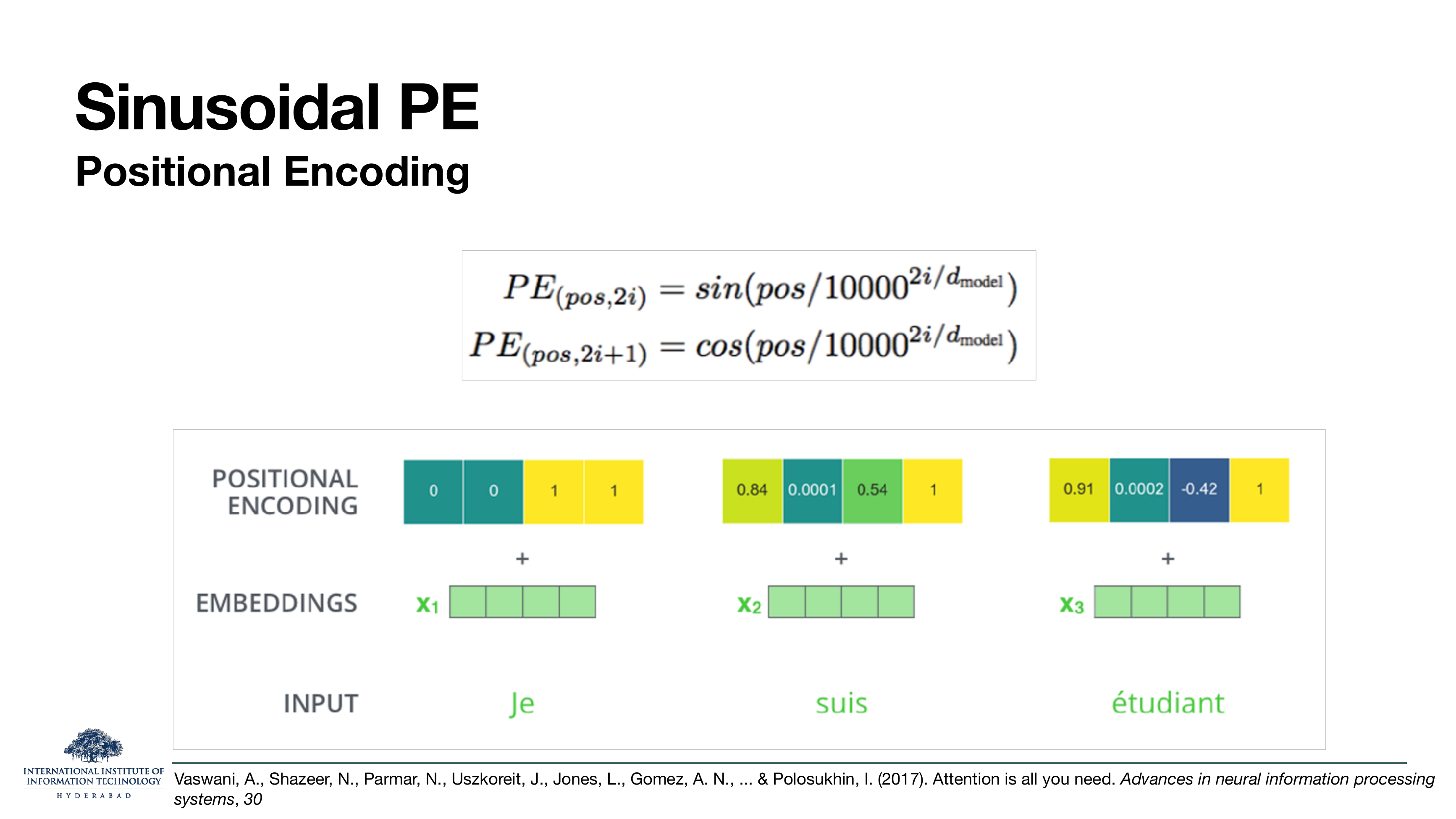
The exact Vaswani formula, then an illustration of it in action on the French phrase Je suis étudiant (I am a student).

PE (pos, 2 i) = \sin (\frac{pos}{10000^{2 i / d_{model}}})

PE (pos, 2 i + 1) = \cos (\frac{pos}{10000^{2 i / d_{model}}})

Reading the formula, dimension by dimension

The positional vector has d_model entries. The even entries get sines, the odd entries get cosines. The frequency of each pair of sine/cosine is $1 / 10000^{2 i / d_{model}}$ — highest at i = 0, and dropping by a factor of 10000 as i walks to the end of the vector. So the first pair of dimensions oscillates very quickly with position (giving the model a fine-grained "which token exactly?" reading), and the last pair oscillates almost not at all (giving a coarse "which region of the sequence?" reading).

What the bottom picture shows

Each of the three input tokens Je, suis, étudiant at positions 0, 1, 2 gets a coloured positional vector. At position 0, sines are 0 and cosines are 1 — you can read the values off the top strip. At position 1 the values shift to (0.84, 0.0001, 0.54, 1); at position 2 they shift again to (0.91, 0.0002, −0.42, 1). The green bars below are the word embeddings x1, x2, x3, and the "+" says these two vectors are summed elementwise. The sum is what enters the transformer.

✦ Key takeaway

Notice the second dimension barely moves (0.0001 → 0.0002). That is the dimension with a very long wavelength — it is meant to distinguish position 0 from position 1000, not position 0 from position 1. Different dimensions carry different "zoom levels" of position.

Slide 10 / 29

Sinusoidal PE Gains: word position; similar performance to learned position embeddings; may allow the model to extrapolate to longer sequences than the ones encountered during training

slide 10 · gains

Slide 11 / 29

Sinusoidal PE Drawbacks: limited generalization to sequence lengths much longer than those seen during training; fixed/pre-defined position, no learnable parameters

slide 11 · drawbacks

What these two slides show

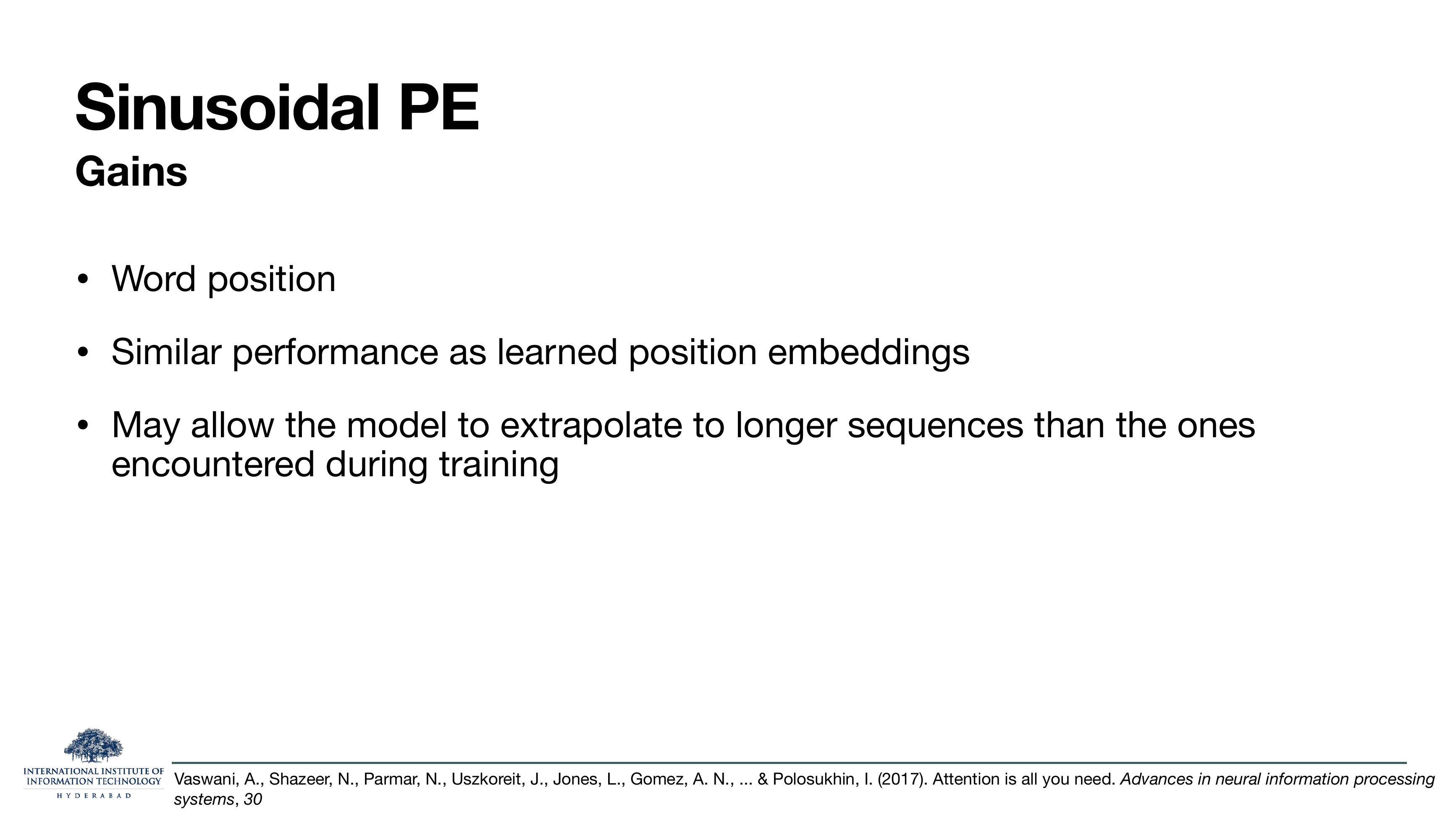
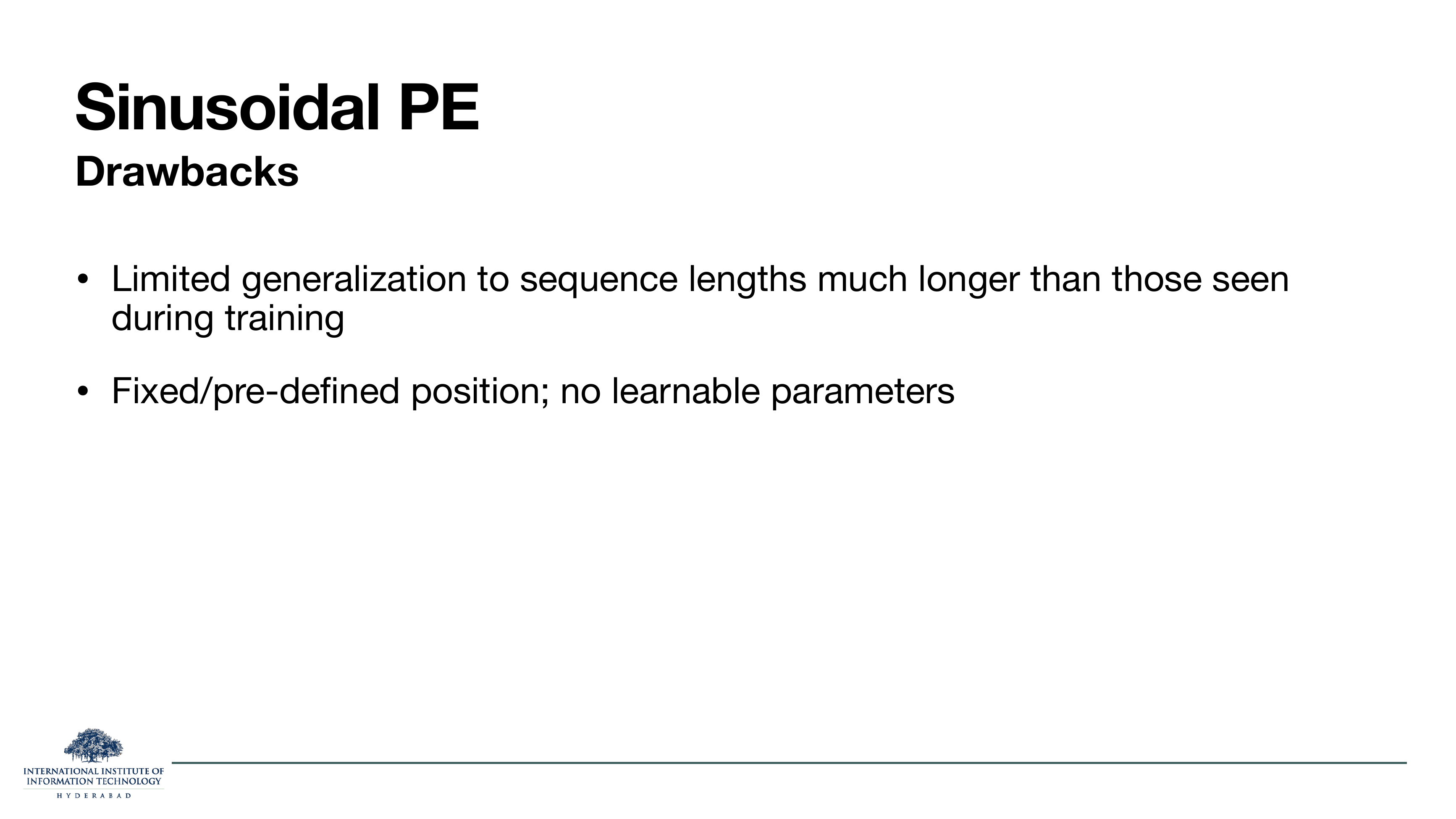
The honest scoreboard for sinusoidal. On the gains side: it gives you a word position at all (so, unlike a bag of words, the model is no longer permutation-blind), it performs about as well as learned absolute embeddings on standard benchmarks, and — the property Vaswani et al. were most excited about — it can in principle extrapolate. Position 513 has a defined vector even if you only trained up to 512.

Why "in principle" is doing a lot of work

The drawback slide corrects the optimism. In practice sinusoidal encodings do compute a well-defined vector for position 513 — but the attention layers above them were only ever trained on positions 0–511, so the downstream behaviour on unseen positions degrades quickly. This turns out to be a general theme, not a sinusoidal-specific bug — most positional schemes generalise poorly to sequence lengths much longer than they were trained on, and a lot of the work in §5 and §6 is about trying to close that gap.

The second drawback is more of a design comment: sinusoidal PE has no learnable parameters. Whether that is good or bad depends on your taste. It saves parameters and removes a source of overfitting, but it also means the model cannot adapt the encoding to the corpus.

§4Relative PE — encode the gap, not the position

Both absolute and sinusoidal encode where a token is. But attention scores really only care about how far apart two tokens are. Shaw et al. (2018) and later T5 (Raffel et al. 2020) pushed this idea to its natural conclusion: instead of adding a position vector to each token, inject a bias directly into the pairwise attention logit — and make that bias a function of the distance between the two tokens.

Slide 12 / 29

slide 12 · section divider

Section divider. Six slides on relative positional encoding — first the general recipe, then T5's specific implementation, then gains and drawbacks.

Slide 13 / 29

Relative PE Approach. Instead of individual token embedding, pairwise embedding. PE calculated between two vectors. Added to self-attention mechanism instead of token vector.

slide 13 · approach

On the slide

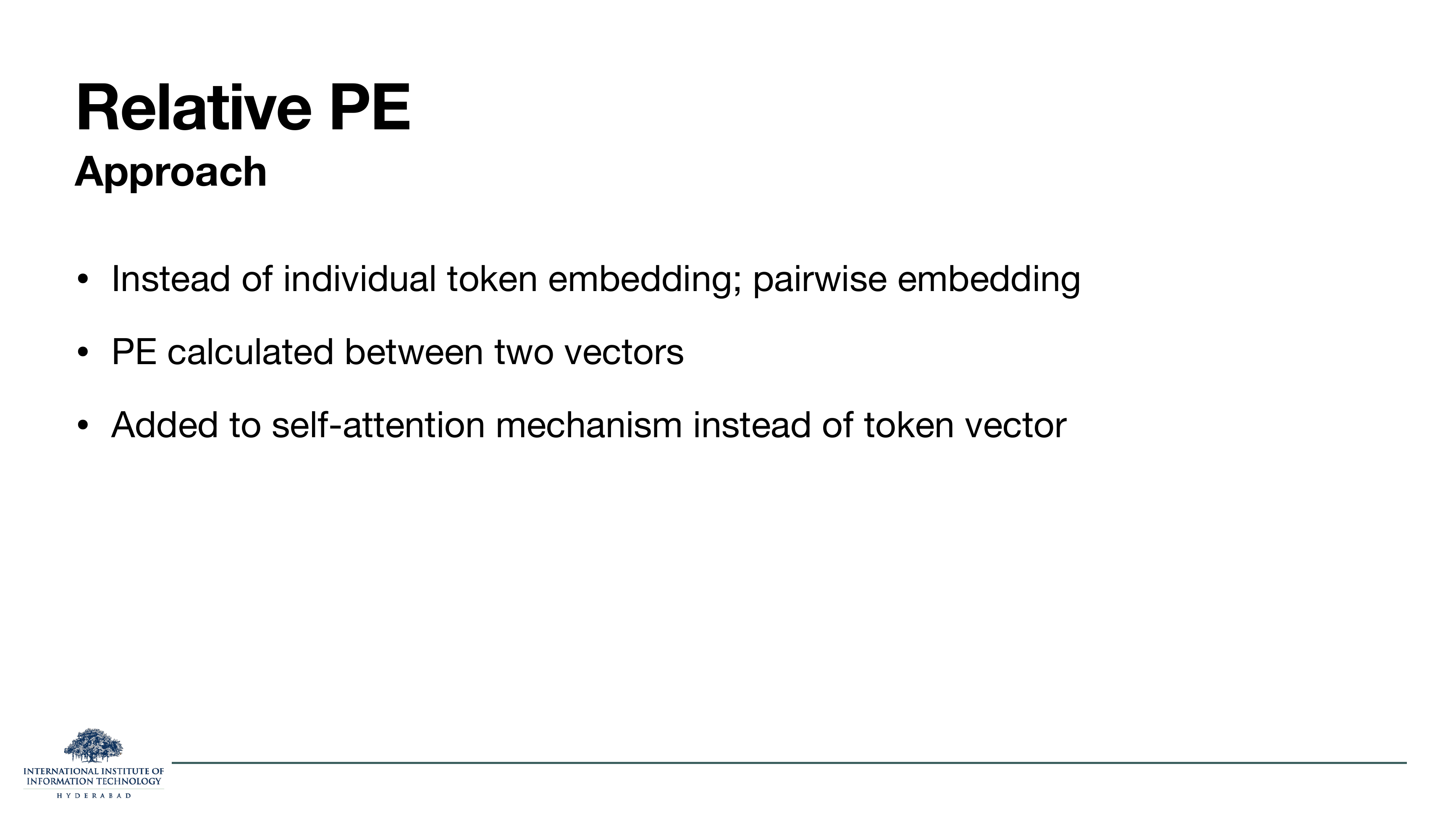
Three bullets that define the shift.

Pairwise, not per-token. A relative PE is not associated with one token — it is associated with a pair: the query at position i and the key at position j. There is one such value for every ordered pair.
Function of the two vectors. More precisely, function of their relative offset i − j.
Injected inside self-attention. Instead of being added to the input embedding, the relative PE is added to the attention logit — the pre-softmax score that says how much query i should attend to key j.

a_{i, j} = \frac{q_{i}^{⊤} k_{j}}{\sqrt{d_{k}}} + b (i - j)

The b(i − j) term is the relative PE. It is a scalar (or, in the general case, a vector) that depends only on the offset.

Slide 14 / 29

Relative PE T5 Approach: simplified form of PE — a scalar is added to the corresponding logit used for computing the attention weights; shared position embedding parameters across all layers; each attention head uses a different learned position embedding. Cites Raffel et al 2020.

slide 14 · T5 approach

Slide 15 / 29

Relative PE T5 Approach continued: 32 embeddings with ranges that increase in size logarithmically up to an offset of 128; beyond, assign all relative positions to the same embedding; given layer is insensitive to relative position beyond 128 tokens; subsequent layers can build a sensitivity to larger offsets by combining local information from previous layers.

slide 15 · T5 buckets

What these two slides show

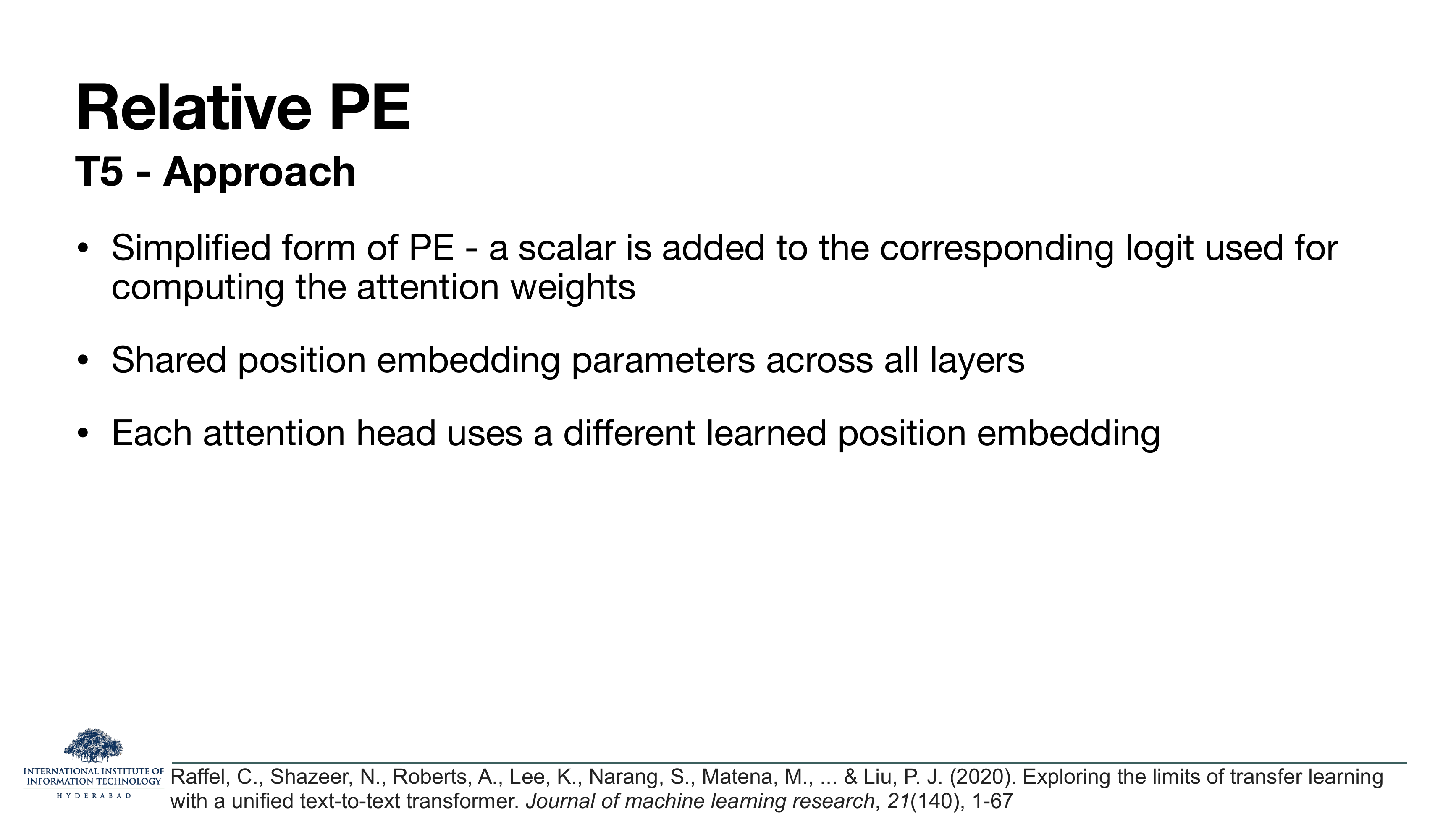
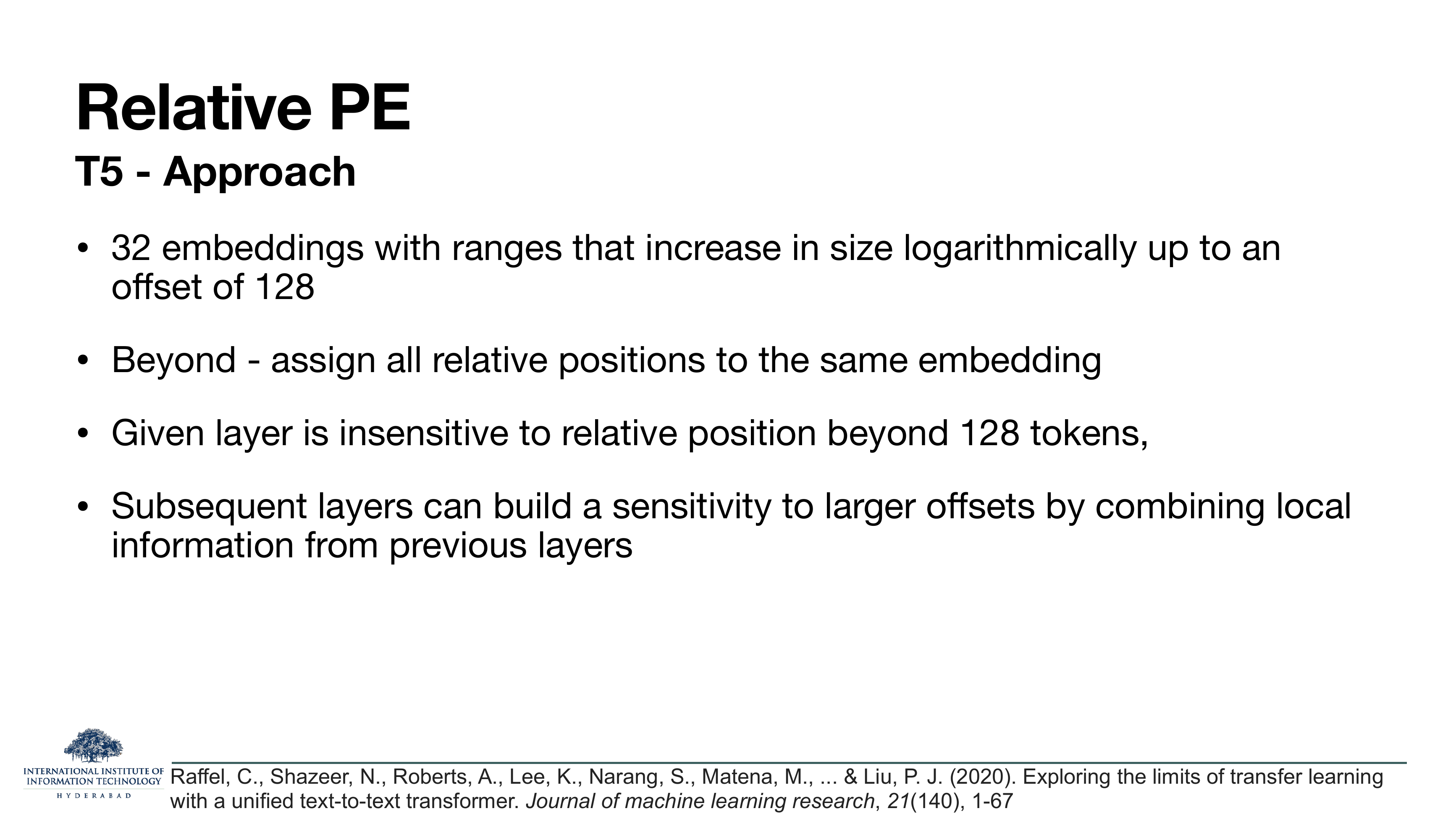
T5's specific way of doing relative PE, in two parts. Slide 14 gives the shape: a single learned scalar per relative offset per attention head, added to the attention logit. The scalar table is shared across all transformer layers but separate per head.

Slide 15 gives the sizing trick. T5 does not learn one scalar per offset up to sequence length — it uses 32 buckets, and the buckets grow logarithmically. Offsets 1, 2, 3, 4 might each get their own bucket. Offsets 5–8 share a bucket. Offsets 9–16 share the next. And so on up to offset 128; everything past 128 shares one big "far away" bucket.

Why bucketise?

Two reasons. First, parameter efficiency: a 32-scalar table per head is cheap regardless of context length. Second — and this is the important one — fine-grained distance only matters when tokens are close. The model needs to distinguish "adjacent" from "2 apart" from "3 apart", because those are typical distances between a word and its head. But the difference between "500 apart" and "501 apart" is almost never linguistically meaningful; both are just "far".

✦ Key takeaway

The last bullet on slide 15 is subtle but important. Even though a single layer is blind to distances past 128, the next layer sees combinations of the previous layer's outputs — and by chaining local reads, a stack of layers can effectively build up a sensitivity to arbitrarily long-range structure. This is the same principle that lets a CNN with 3×3 kernels see the whole image after enough layers.

Slide 16 / 29

Relative PE Gains: enhanced representation; better generalization at varied sequence length

slide 16 · gains

Slide 17 / 29

Relative PE Drawbacks: implementation complexity; delay in training and inference; can't cache — compute new key-value pairs for every new token

slide 17 · drawbacks

What these two slides show

The scoreboard for relative PE. On the plus side: varied sequence length is handled naturally — the encoding is a function of the offset, and offsets don't depend on absolute sequence length. Train on 512, test on 1024, and the model still knows what "3 apart" means.

On the minus side, three practical costs.

Implementation complexity. A per-pair bias means an O(L²) tensor of biases per layer. Efficient implementations need care — you don't want to materialise the full L × L matrix if you don't have to.
Training/inference latency. The extra add is cheap but non-zero, and it lands on the critical path of every attention op.
KV-cache invalidation. This is the biggest one and the reason relative PE fell out of fashion for large autoregressive LMs. In a decoder-only LM you cache the keys and values of previous tokens so you don't recompute them at each step. But with relative PE, when a new token arrives, the bias b(i − j) for existing keys shifts — because i just changed. So you cannot simply reuse the cached keys and values as they are; you have to recompute the attention logits. This is a serious performance tax on generation.

→ Keep reading

RoPE (§5) was designed specifically to fix the caching problem while keeping the relative-position feel of T5. It succeeds so well that essentially every modern LLM — LLaMA, Qwen, Mistral, DeepSeek — uses it.

§5RoPE — rotate the query and key

Rotary Position Embedding (Su et al., 2021) is the answer that took over. The trick is elegant. Instead of adding a positional vector to the input, or a scalar bias to the logit, RoPE rotates the query and key vectors in the complex plane by an angle proportional to their position. When you then take the dot product q·k, the rotation angles combine into a difference — so the dot product ends up depending only on the relative position, while each vector still knows its own absolute position. Seven slides to work through the picture, the algebra, and the payoff.

Slide 18 / 29

slide 18 · section divider

Section header for RoPE — Rotary Position Embedding.

Slide 19 / 29

RoPE Approach: integrate positional information into the learning; encodes absolute position with a rotation matrix; incorporate the explicit relative position dependency in self-attention formulation; rotate the affine-transformed word embedding vector by amount of angle multiples of its position index. Introduced in 2021. Cites Su et al 2024 Roformer paper.

slide 19 · approach

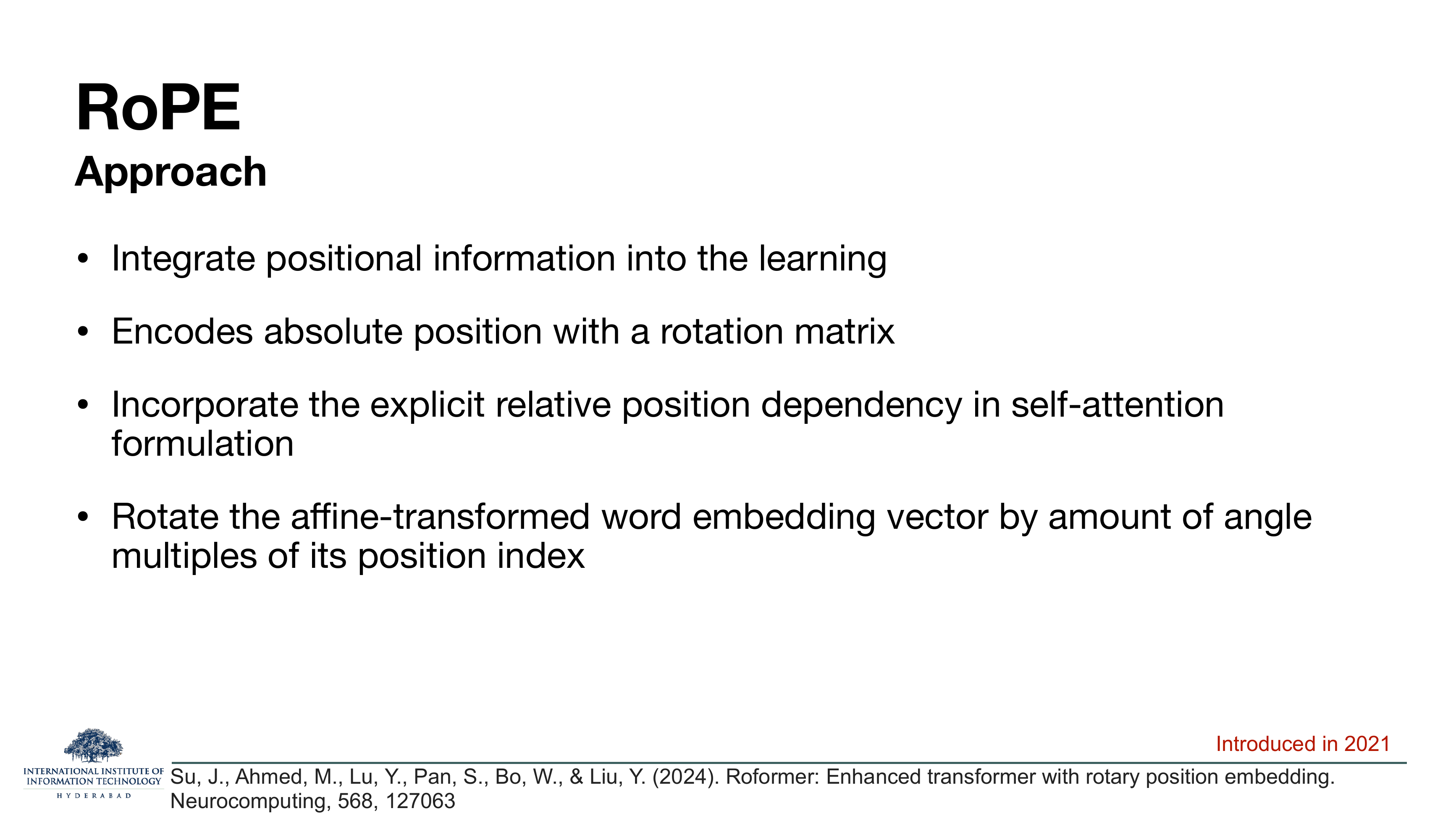
On the slide

Four one-line claims that together describe what RoPE does.

Position is not a table lookup added at the input; it is baked into the attention computation itself.
Absolute position is encoded via a rotation matrix.
The design ensures the dot product query·key ends up depending on the relative offset between the two positions.
Concretely: take the query (or key) vector after its usual affine projection, and rotate it by an angle that is a multiple of the position index.

The paper is RoFormer: Enhanced Transformer with Rotary Position Embedding, Su et al., first arXiv release in 2021, published in Neurocomputing 568 (2024).

✦ Key takeaway

RoPE is the rare design that lets you have both. Absolute position is in the vector (each token's rotation angle depends only on its own position). Yet when two rotated vectors are dot-producted, the answer turns out to depend only on the difference of their positions — the individual angles cancel out into a relative angle. Best of both worlds, and it also plays nicely with KV-caching because a cached key at position j keeps its rotation forever.

Slide 20 / 29

RoPE Implementation diagram: top panel shows a 2D example where a query/key pair (x1, x2) is rotated by angle m*theta_1 into (x1', x2'). Bottom panel shows a stack of six token embeddings — Enhanced Transformer with Rotary Position Embedding — with each embedding being rotated by an angle proportional to its position 1 through 6.

slide 20 · the picture

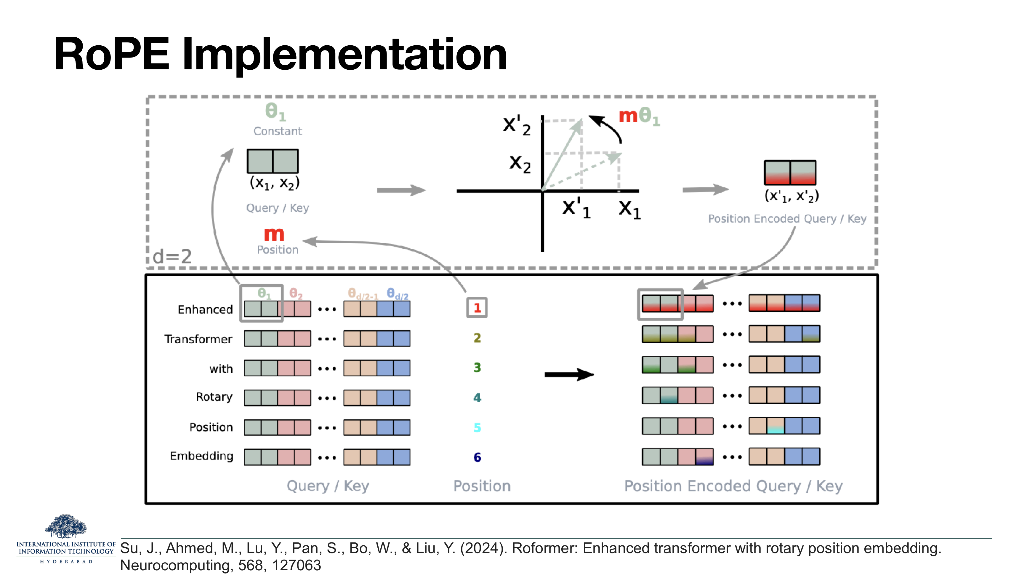
On the slide

The RoPE mechanism in one figure. Take the query or key vector (x1, x2). Rotate it in the plane by angle m · θ₁ — where m is the token's position index and θ₁ is a fixed frequency for this pair of dimensions. Call the rotated vector (x'₁, x'₂). That is your position-encoded query or key.

The bottom panel shows the same recipe applied to a full six-token sentence — "Enhanced Transformer with Rotary Position Embedding", positions 1 through 6. The tinted colour on each output vector represents the accumulating rotation. Position 1 gets a small twist. Position 6 gets a large one.

How the "d dimensions" generalise the 2D picture

The query and key vectors are d-dimensional, not 2-dimensional. RoPE splits the d dimensions into d/2 consecutive 2D pairs. Each pair gets its own frequency θᵢ — high frequencies for the first pairs, low frequencies for the last, in the same 10000^−2i/d style as the sinusoidal formula. Each pair is rotated independently by the position-dependent angle for that frequency.

Slide 21 / 29

$RoPE Approach 2D example: complex-form equations f_q(x_m, m) = (W_q x_m) e^{im theta}, f_k(x_n, n) = (W_k x_n) e^{in theta}, g(x_m, x_n, m-n) = Re[(W_q x_m)(W_k x_n)* e^{i(m-n)theta}]. Below: the same operation in real form as a 2x2 rotation matrix times the affine projection.$

slide 21 · 2D algebra

Slide 22 / 29

$RoPE general form: f_{q,k}(x_m, m) = R^d_{Theta, m} W_{q,k} x_m where R^d_{Theta, m} is a block-diagonal rotation matrix with 2x2 rotation blocks for angles m*theta_1, m*theta_2, ..., m*theta_{d/2}. Rotary matrix with pre-defined parameters Theta = {theta_i = 10000^{-2(i-1)/d}, i in [1,2,...,d/2]}.$

slide 22 · the full matrix

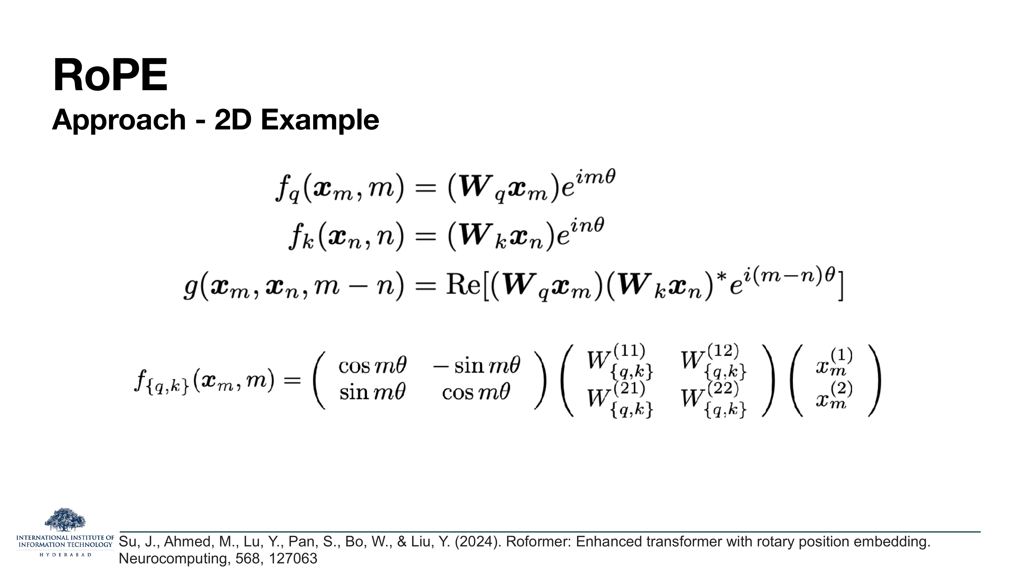
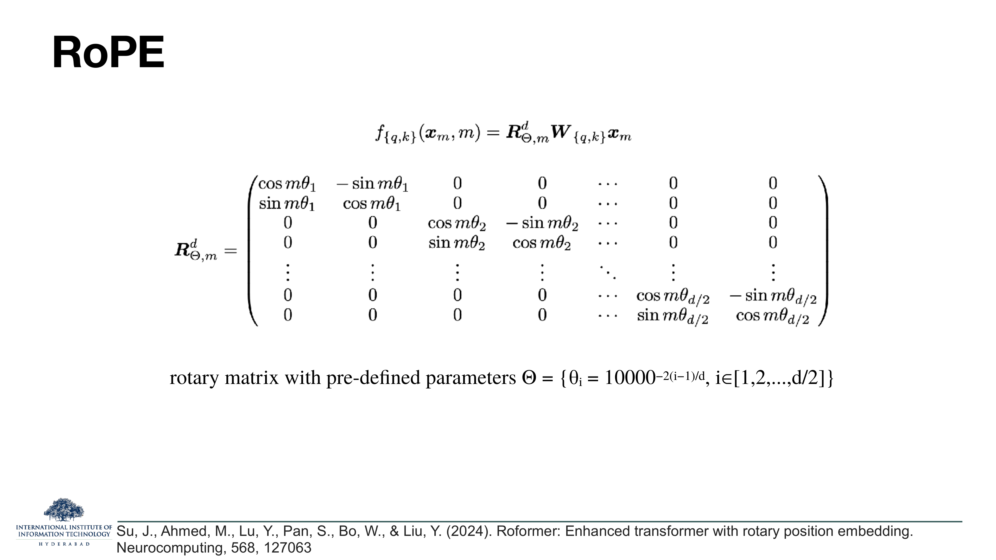
What these two slides show

Slide 21 is the derivation in complex form and the 2D real form. Represent each 2D slice of the vector as a complex number. Then rotating by angle m·θ is just multiplying by e^imθ. So the position-encoded query for token at position m is

f_{q} (x_{m}, m) = (W_{q} x_{m}) e^{i m θ}

and similarly for the key at position n. When you form the inner product, $e^{i m θ} \cdot e^{- i n θ} = e^{i (m - n) θ}$ — the answer only depends on m − n. That is the whole point.

Slide 22 promotes the 2D picture to d dimensions. The rotation acts as a big block-diagonal matrix $R_{Θ, m}^{d}$ , where each 2×2 block on the diagonal is a standard rotation by angle m·θᵢ. The frequencies θᵢ are pre-defined the same way as in sinusoidal PE:

θ_{i} = 10000^{- 2 (i - 1) / d}, i \in [1, 2, \dots, d / 2]

⚠ Watch out

The rotation matrix looks huge but you never actually build it. In code, RoPE is applied by taking pairs of adjacent dimensions (x_2i, x_2i+1) and computing (x_2icos φ − x_2i+1sin φ, x_2isin φ + x_2i+1cos φ) with φ = m·θᵢ. That's it — one pair of trig multiplies per pair of dimensions, no matrix ever materialised.

Slide 23 / 29

RoPE Gains: flexibility of sequence length; decaying inter-token dependency with increasing relative distances; capability of equipping the linear self-attention with relative position encoding; interpretability — rotational approach offers intuitive geometric interpretation of how positional information influences the attention mechanism

slide 23 · gains

Slide 24 / 29

RoPE Drawbacks: implementation complexity

slide 24 · drawbacks

What these two slides show

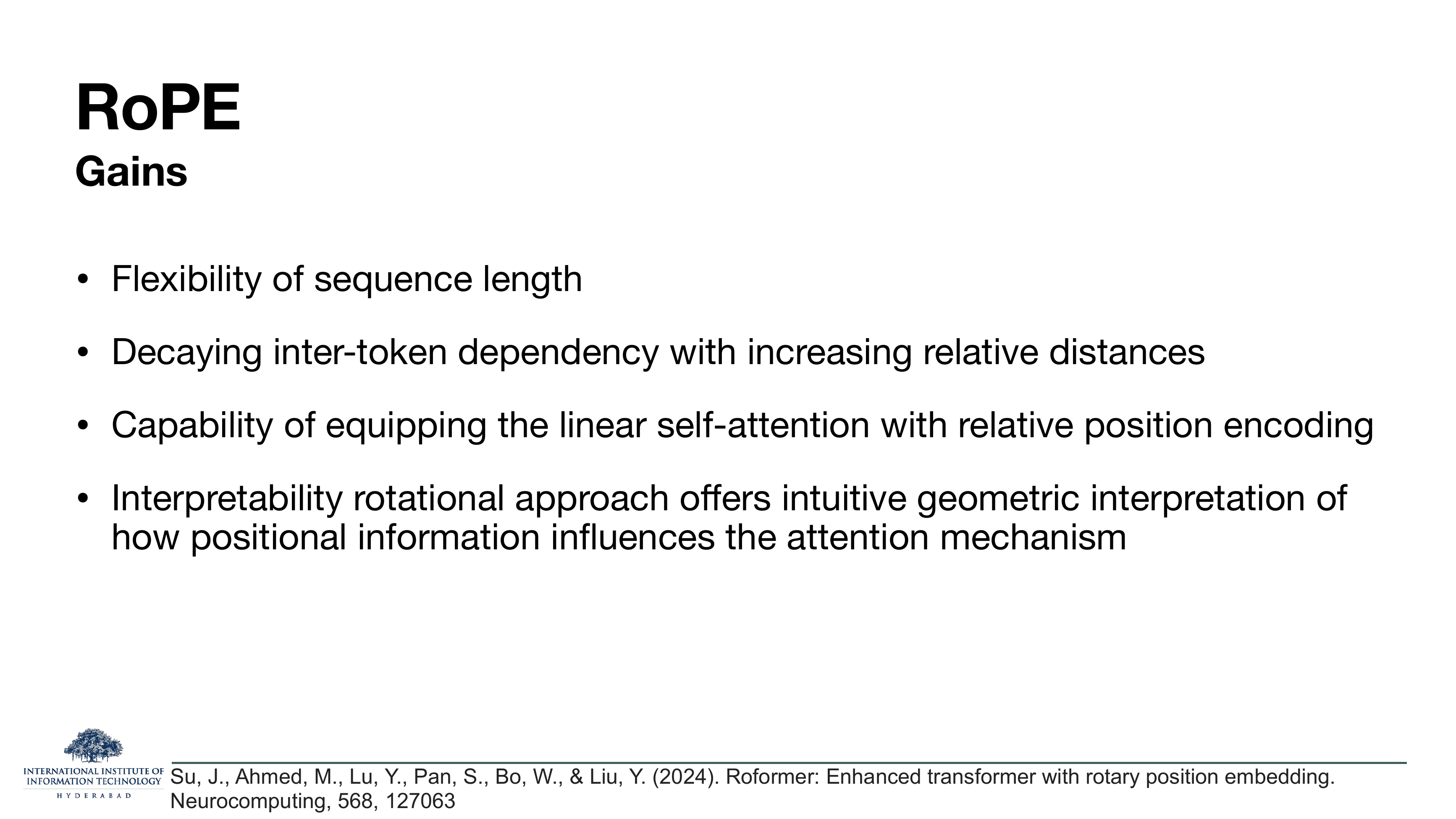
RoPE's scoreboard. Four gains, one drawback.

Flexibility of sequence length. Nothing in the design assumes a maximum sequence length — you can encode position 100,000 as easily as position 5. The attention behaviour at position 100,000 is only as good as the training data, but the encoding itself never runs out of vectors.
Decaying inter-token dependency. Because different dimension-pairs rotate at different rates, the inner product of two rotated vectors naturally decays as the offset |m − n| grows — high-frequency pairs oscillate quickly and average out, low-frequency pairs stay coherent. So RoPE gives you a built-in "closer tokens matter more" inductive bias, without you having to hand-code it.
Works with linear-attention variants. Because RoPE is applied to the queries and keys directly (not injected into the softmax bias), it composes cleanly with linear-attention and other efficient-attention recipes that don't touch the softmax at all.
Interpretability. Rotations have a picture — you can literally see position as angle. This makes RoPE the easiest positional scheme to reason about qualitatively.

The single drawback is honest: implementation complexity. It is not free code. You need to interleave sin/cos multiplies at the right place in the attention forward pass, and getting the dimension pairing right (adjacent pairs, or the split-half convention some frameworks use) is a common source of bugs.

→ Keep reading

Practically every LLM you have heard of from 2023 onwards — LLaMA, Qwen, Mistral, DeepSeek, Gemma, Phi — uses RoPE. Later work (YaRN, NTK-aware scaling, position interpolation) extends RoPE to context lengths far beyond what it was trained on, but the core recipe is unchanged.

§6NoPE — maybe you didn't need any of this

The last section is a plot twist. Kazemnejad et al. (2023) asked a stubborn question: what happens if you remove the positional encoding entirely? The result — for decoder-only, causally masked models — is surprising. The model still learns to use word order, apparently because the causal mask itself carries enough asymmetry that gradient descent can reconstruct positional information without any explicit encoding. Five slides on this finding and its consequences for current frontier models.

Slide 25 / 29

slide 25 · section divider

Section header. NoPE stands for No Positional Encoding — the deliberate choice to omit any explicit position signal.

Slide 26 / 29

NoPE Approach: no explicit positional embedding — not fixed, learned, or relative; causal mask gives autoregressive model an implicit sense of order; model learns to exploit the asymmetry to reconstruct positional information on its own via SGD. Cites Kazemnejad et al 2023.

slide 26 · approach

Slide 27 / 29

NoPE Approach: causal mask — a token at position t can only see tokens at positions ≤ t; implicit sense of direction; regular gradient-descent-based training learns to exploit it if it finds it beneficial for the optimization objective; when trained with SGD it mostly resembles T5's relative PE attention patterns.

slide 27 · the mechanism

What these two slides show

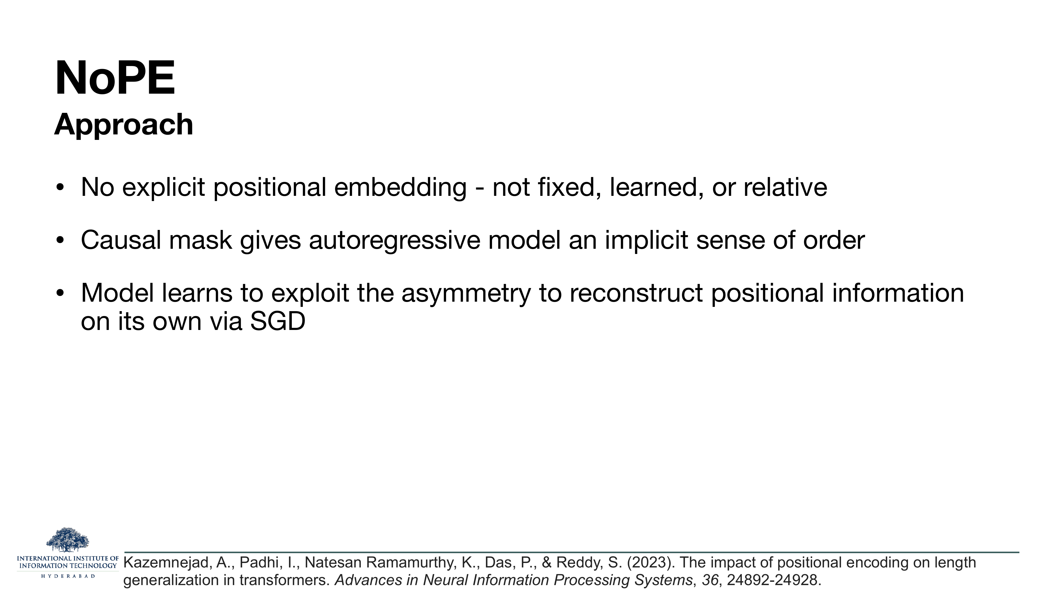
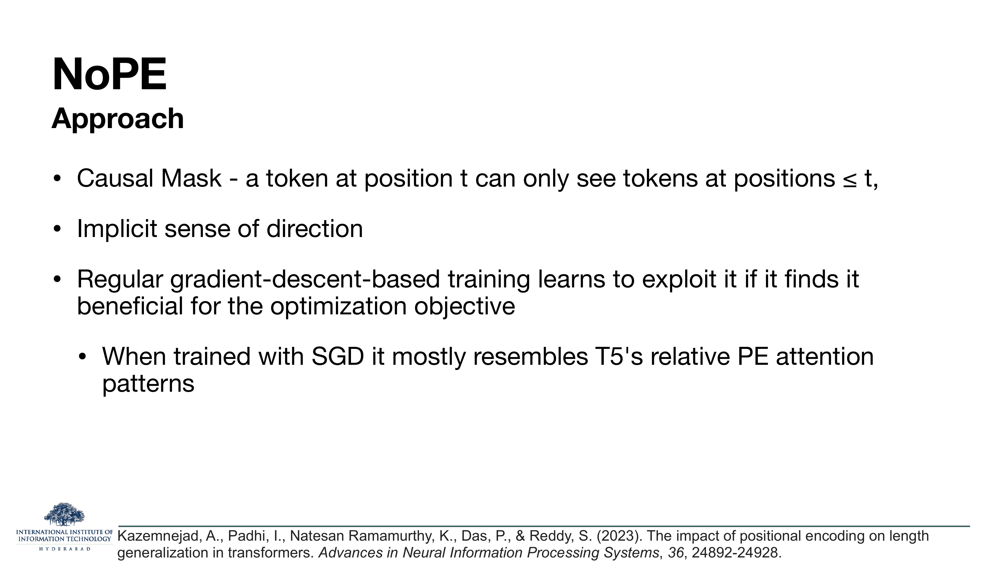
The NoPE claim and its justification, over two slides.

Slide 26 puts it as sharply as possible. There is no positional signal in the input at all — not absolute, not sinusoidal, not relative, not RoPE. Yet the model still learns to use word order. The reason: the causal mask in a decoder-only transformer is itself an asymmetric operator. A token at position t can attend only to tokens at positions ≤ t, never in the other direction. The set of tokens visible to token 0 is a strict subset of the set visible to token 1, which is a strict subset of the set visible to token 2, and so on. Any position-sensitive computation the model wants to do — counting how many tokens are on the left, or measuring recency — can be assembled out of that asymmetry.

Slide 27 spells out the mechanism. Since gradient descent will exploit any structural asymmetry that helps the loss, and since the causal mask is such an asymmetry, the model organically learns to route positional information through the attention pattern. The paper's striking empirical finding is that the resulting attention patterns end up looking a lot like T5's relative-position patterns — meaning the model has essentially reinvented relative PE from the mask alone.

✦ Key takeaway

Note the "causal mask" qualifier. NoPE does not work for encoder-only models (BERT-style) with bidirectional attention — there the attention operation is fully symmetric, and without a positional signal the model really is order-blind. NoPE is a phenomenon of decoder-only LMs. Which, conveniently, is what almost all modern frontier LLMs are.

Slide 28 / 29

NoPE Approach — Current Models: SmolLM3 uses a mixed design and omits RoPE in every fourth layer; Kimi applies NoPE in its MLA global-attention layers; this lets MLA run as pure multi-query attention at inference and avoids RoPE retuning for long-context scaling; Kimi K3 uses only NoPE, no RoPE layers at all.

slide 28 · NoPE in the wild

On the slide

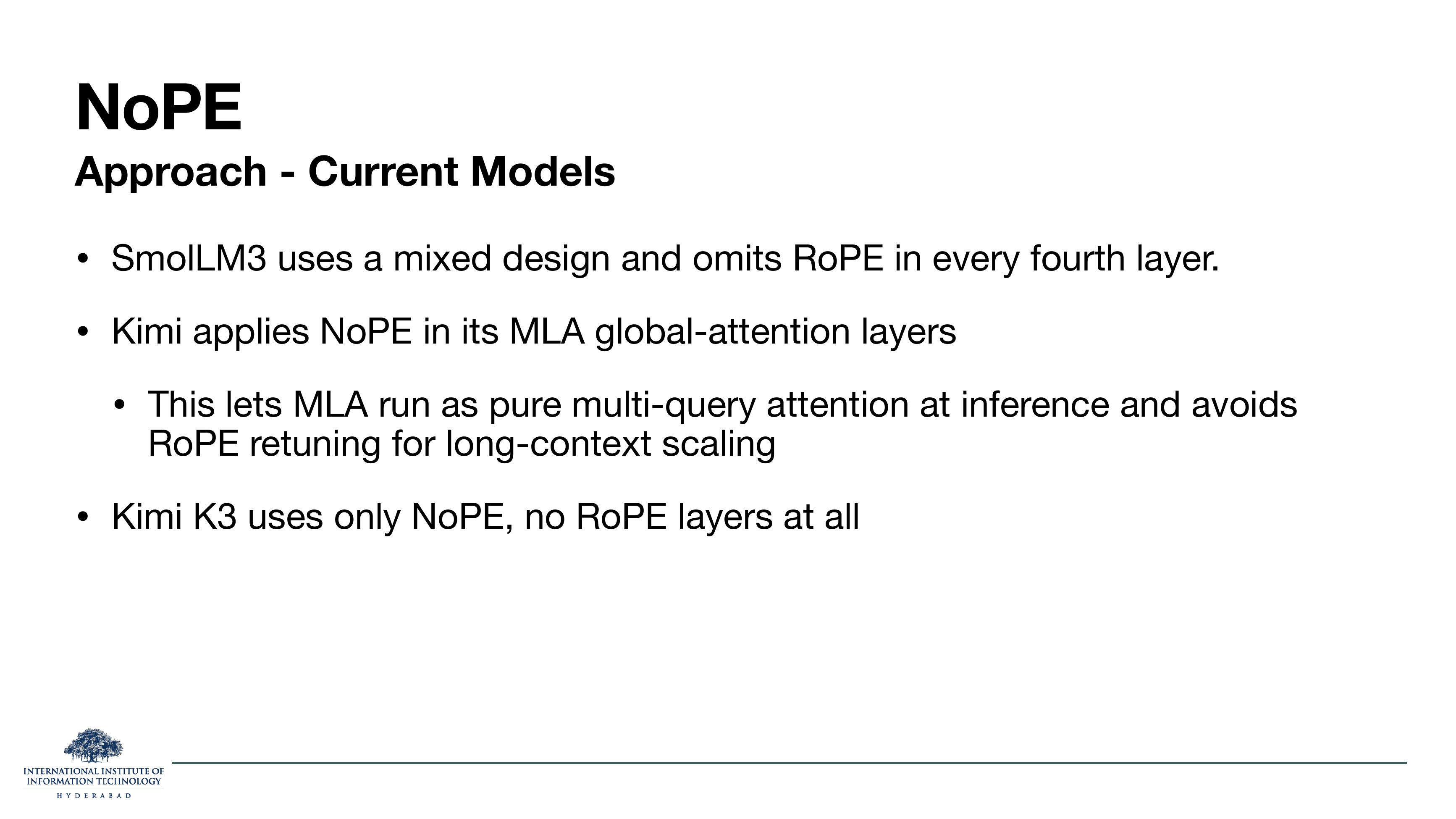
Three current frontier-scale examples of NoPE being used in production, not just as an academic curiosity.

SmolLM3. HuggingFace's small-model line uses a mixed design: RoPE in three out of every four layers, NoPE in the fourth. The idea is that a handful of position-agnostic layers act as a long-range "escape hatch" while the RoPE layers still handle local structure.
Kimi (Moonshot AI). Kimi's Multi-head Latent Attention (MLA) uses NoPE in its global-attention layers. The practical payoff is that MLA can then run as a plain multi-query attention at inference — the KV cache is small and simple — and the model doesn't need any of the RoPE-retuning tricks (YaRN, position interpolation) usually required to push RoPE past its training length.
Kimi K3. Goes all the way: no RoPE anywhere. Pure NoPE across the whole stack. This is the strongest bet on Kazemnejad et al.'s finding to date at scale.

→ Keep reading

The long-context scaling story is really the point. Every RoPE-based model that wants to serve 100k+ tokens has to retune the RoPE frequencies (YaRN, NTK-aware scaling, position interpolation), and each retuning is a small research project. NoPE sidesteps all of that: nothing to retune, because there was nothing tuned in the first place.

Slide 29 / 29

NoPE Gains: simple — no additional computation; generalizes to longer sequences better than RoPE or absolute embeddings; theoretically can represent both absolute and relative positional encodings

slide 29 · gains

On the slide

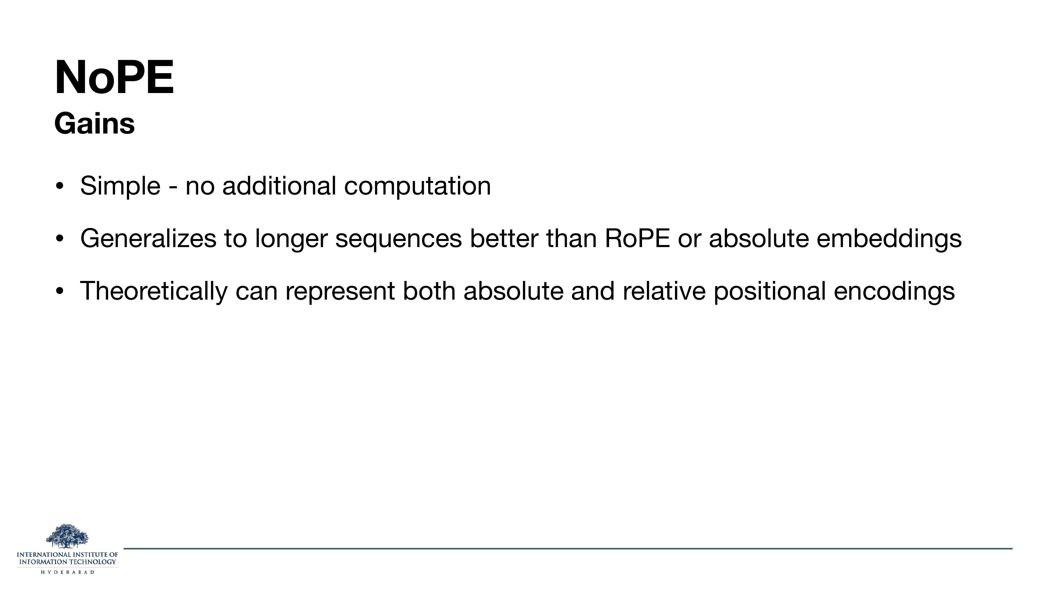
The scoreboard for NoPE. Three gains, and no explicit "drawbacks" slide — the deck ends here.

Simplicity. Zero extra computation. Zero extra parameters. No sin/cos multiplies in the attention path. Nothing to tune.
Length generalisation. Kazemnejad et al.'s central empirical finding: on synthetic length-extrapolation tasks, NoPE actually outperforms RoPE and absolute embeddings at sequence lengths well beyond training. Nothing in the model breaks at position 4097 because nothing in the model ever knew about the number 4096.
Theoretical expressivity. The paper proves that a NoPE transformer can, in principle, represent both absolute and relative positional encodings via its learned attention patterns — so nothing you could express with RoPE is out of reach.

⚠ Watch out

NoPE is not "positional encoding was a mistake". Bidirectional encoders (BERT, ViT with global attention) still need it. And even in decoder-only models, RoPE and NoPE tend to trade off differently on short-context tasks vs. long-context extrapolation — NoPE isn't uniformly better, it's better at length generalisation. Which is why designs like SmolLM3 mix both.

✦ the deck's punchline

Look at where the story has gone. Slide 5: learned position lookup. Slide 9: fixed sinusoidal function. Slide 14: pairwise bias on the logit. Slide 22: rotation of query and key. Slide 26: nothing. Each step removed a piece of the mechanism and asked "did we actually need it?", and the answer, more often than the original transformer paper would have guessed, was no. The direction of travel in the field is toward less hand-designed structure, not more.