Lecture 06 · 21 slides · September 3, 2026

More Attention: the variants that make it fit.

Standard attention lets every token compare itself with every other token, which means building an n-by-n score matrix at every layer. Doubling the context therefore quadruples the work. This lecture covers two responses: compute fewer pairs with sliding, sparse, or BigBird attention, or avoid materializing the matrix with linear attention.

Lecture 06 21 slides Manish Shrivastava · Aparajitha Allamraju

§0The deck at a glance

The lecture begins with the quadratic cost of standard attention, then compares sliding, sparse, and BigBird masks. The final section changes the attention computation itself to make cost linear in sequence length. For each method, track the mask, KV-cache cost, and what the efficiency gain gives up.

§1The O(n²) problem

The two slides that frame the whole lecture. Slide 1 is the title card; slide 2 is a small but load-bearing list of what standard attention costs you.

Slide 01 / 21

Title slide: More Attention, Advanced NLP M26, IIIT Hyderabad, September 3 2026

slide 01 · title

On the slide

Lecture 6 of Advanced NLP, Monsoon 2026. The title More Attention is a promise: you already know one attention (the one from Lecture 5). Now you get four more, each one designed to fix something that scaled dot-product attention is bad at.

What to take from it

The transformer's ubiquity is partly an accident of hardware. Attention was picked in 2017 because it parallelised on GPUs. Its quadratic cost in the sequence length was tolerated back then because sequences were short (128 to 512 tokens). The moment people wanted 32k, 128k, or 1M-token contexts, that quadratic became the bottleneck of the entire field. This lecture is how the field responded.

Slide 02 / 21

Standard Attention / Scaled Dot-Product Attention. Disadvantages: quadratic in time; every token attends to every other; fixed context window limits input size.

slide 02 · why standard attention hurts

On the slide

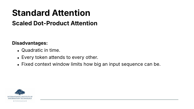
Three disadvantages of scaled dot-product attention, the operation from Lecture 5 that computes $softmax (\frac{Q K^{⊤}}{\sqrt{d_{k}}}) V$ . The three complaints are linked, not independent.

What to take from it

The middle bullet, every token attends to every other, is the cause; the other two are symptoms. If every one of n queries dot-products against every one of n keys, you build an n×n matrix. That matrix takes $O (n^{2})$ arithmetic and $O (n^{2})$ memory. So you cannot afford long n, and that is where the "fixed context window" ceiling comes from.

✦ Key takeaway

Every variant in the rest of the lecture is a way of saying no, my query does not need to look at every key. Sliding attention says "only my neighbours." Sparse says "only a striped subset." BigBird says "neighbours plus a few globals plus a bit of random." Linear says "look at all of them, but through a factorisation that never materialises the matrix." Same disease, four different medicines.

→ Background

The disease itself is introduced in Lecture 5. If any symbol here (Q, K, V, softmax, KV cache) is unfamiliar, go back and skim slides on scaled dot-product attention before continuing.

§2Sliding-window attention: attend to your neighbours

The simplest fix. Instead of letting a query look at all n keys, let it look only at a window of w keys centred on itself. The mask stops being a full square and becomes a thin band down the diagonal. This is the idea behind Longformer (Beltagy, Peters, and Cohan, 2020), the first paper to make long-document transformers practical.

Slide 03 / 21

Sliding Attention: attends to neighbours in a window; linear in input and window; stacking enables distant influence. Four heatmaps: full n^2, sliding window, dilated sliding, and global+sliding.

slide 03 · Longformer's four patterns

On the slide

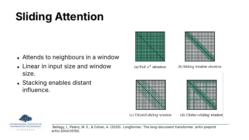
Four attention masks from the Longformer paper. In each, the axes are query index (rows) and key index (columns), and green cells are the (query, key) pairs that are actually computed:

(a) Full n² attention. The standard mask, a solid green square. Everyone looks at everyone.
(b) Sliding window. A thin diagonal band of width w. Each query attends to w/2 tokens on either side.
(c) Dilated sliding window. The same band, but with gaps: skip every other key. This widens the receptive field without adding cost, the same trick that WaveNet uses in dilated convolutions.
(d) Global plus sliding. The band, plus a few full rows and columns for global tokens (typically [CLS] or question tokens) that every position attends to and that attend to everything.

What to take from it

Instead of an n×n matrix, you keep an n×w band. Cost drops from $O (n^{2})$ to $O (n w)$ , which is linear in n when w is fixed. And the third bullet, "stacking enables distant influence", is the honest defense of this design: a token can only reach w/2 neighbours in one layer, but after L layers its receptive field is L·w/2, so with enough depth it can still influence a distant token indirectly, the way information flows across a CNN.

Under the hood

Every family in this lecture reduces to which cells of the attention matrix do I actually compute. Sliding attention is the case where the answer is a band of width w. All the arithmetic tricks follow from that mask.

Slide 04 / 21

Sliding Attention Limitations: long-range interaction requires many stacked layers; W too small loses information, W too large defeats the purpose.

slide 04 · sliding limitations

On the slide

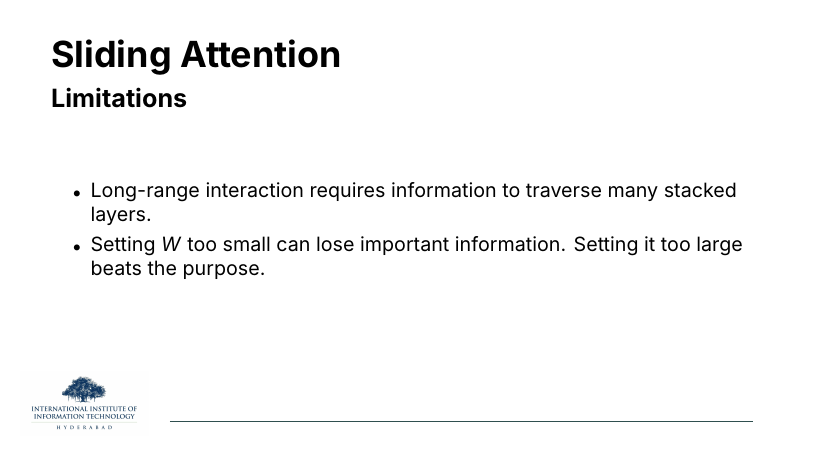
The honest downsides. Two of them.

What to take from it

The first is the CNN problem in disguise: to relate token 1 to token 10 000 you need $10000 / (w / 2)$ layers of message-passing. Depth is not free.

The second is a tuning trap. Small w and you drop important long-range signal; large w and you are back paying for something close to full attention.

Slide 05 / 21

Sliding Attention memory table: d=2048, n=2048, d_h=128, h=l=16, w=128. K/Q/V params, and KV cache is w·l·2·d_h = 0.03 MParams / 4 MB per token.

slide 05 · sliding memory table

On the slide

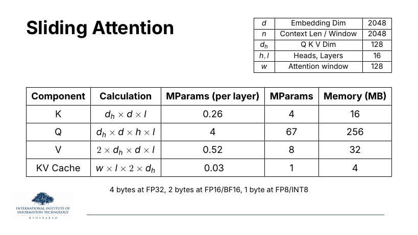
A worked memory table for a reference model: 2048-dim embeddings, 16 heads, 16 layers, and a window of w = 128 tokens. The KV cache row is the punchline: because each layer only needs to remember the last w keys/values, the cache is $w \cdot l \cdot 2 \cdot d_{h}$ per token: a fixed 4 MB, not a growing quantity.

Why the KV cache row matters

The KV cache is what a decoder keeps in GPU memory during generation so that the next token can attend to the past without recomputing keys and values. In standard attention it grows linearly with the number of generated tokens; here it is capped at w. That is the practical reason people ship sliding attention: it makes inference at 100k tokens fit on one card.

§3Sparse attention: attend to a chosen few

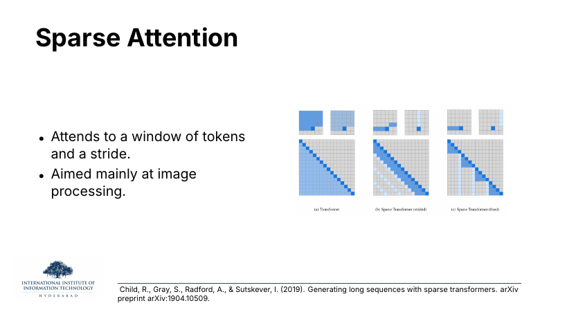
Sliding is one way to sparsify, but it is not the only pattern that works. Slide 6 introduces the Sparse Transformer of Child et al. (2019), which keeps a small stride of long-range connections in the mask. Slide 8 fast-forwards to DeepSeek-v3.2's idea: rather than fix the sparsity pattern, learn which past tokens are worth keeping, per query.

Slide 06 / 21

Sparse Attention: attends to a window of tokens and a stride; mainly aimed at image processing. Three attention patterns: (a) full transformer, (b) sparse strided, (c) sparse fixed.

slide 06 · Child et al. sparse patterns

On the slide

Three masks from the Sparse Transformers paper. The full pattern (left) is compared to two structured sparsifications. Strided: attend to your local window and every k-th token in the past. Fixed: attend to your window and to a fixed set of "summary" positions.

What to take from it

The design intent was image generation: the paper factorises attention into two heads that between them cover the full 2D image raster in $O (n \sqrt{n})$ instead of $O (n^{2})$ . One head handles the local neighbourhood; the other jumps a fixed stride so that after two hops any pixel can reach any other.

→ where the note comes from

"Aimed mainly at image processing" is a historical note. Pixel neighbourhoods have strong local structure and a natural stride (row width), which is exactly what strided sparse patterns exploit. For text the payoff is smaller, and that is one reason BigBird added random links on top.

Slide 07 / 21

Sparse Attention memory table with the same reference numbers as sliding: KV cache is w·l·2·d_h = 0.02 MParams / 4 MB.

slide 07 · sparse memory (fixed w)

On the slide

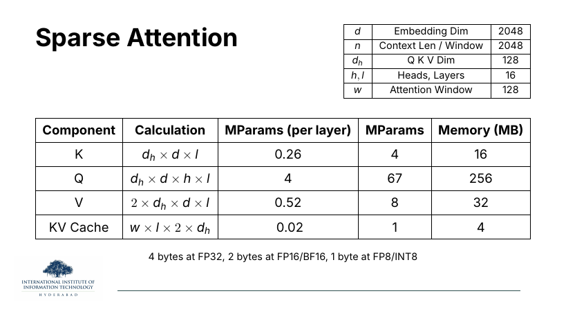
The same reference model as slide 5. The parameter columns don't change: the projections Q, K, V are the same whatever the mask does. What changes is the KV cache, still ~4 MB per position because each query only needs its window of past keys and values in fast memory.

Why the tables look almost identical

These memory tables recur through the lecture on purpose. Each family costs roughly the same in parameters; the differences are in the cache and in the arithmetic per step. The savings come from what you don't compute, not from what you don't store as weights.

Slide 08 / 21

Sparse Attention (DeepSeek): attends to a selected few tokens with no window; selected few are top-k attention scores in a specialised low-precision head.

slide 08 · DeepSeek top-k selection

On the slide

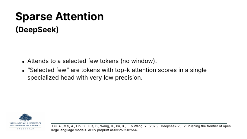
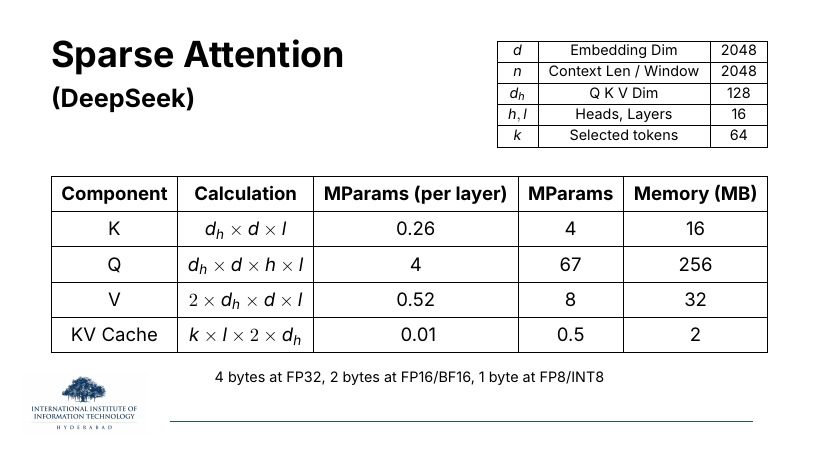
DeepSeek-v3.2's contribution to sparse attention. There is no window at all. For each query, a tiny specialised "index" head (run at very low precision to keep it cheap) scores all past tokens; only the top-k highest scorers get promoted to full-precision attention.

What to take from it

Fixed masks (windows, strides) are a guess about where attention wants to look. DeepSeek's move is to ask, cheaply, then look only at the winners. This is a form of learned sparsity: the mask is dynamic, per-query, per-layer.

Under the hood

Think of it as a two-stage attention. Stage 1: a lightweight, low-precision "lightning attention" scores every past token; this is cheap because the scores are approximate and never fed to softmax. Stage 2: sort those scores, take the top k, and do real attention over just those k. Total cost is roughly $O (n k)$ plus the cheap indexing pass.

Slide 09 / 21

Sparse (DeepSeek) memory table with k=64 selected tokens: KV cache k·l·2·d_h = 0.01 MParams / 2 MB — half the sliding cost.

slide 09 · DeepSeek memory (selected k)

On the slide

Same reference model as before, with one changed row in the parameter table: k = 64 selected tokens per query. The KV cache is now $k \cdot l \cdot 2 \cdot d_{h}$ , which is 2 MB per position, half of what a sliding window of 128 costs.

Why keep this in mind

Fewer tokens attended to means less to keep in cache and less arithmetic. The reason DeepSeek can afford k = 64 while sliding needed w = 128 is that the 64 are chosen adaptively. You spend your budget on the tokens the query actually cares about, not on whichever tokens happen to sit next to it.

Slide 10 / 21

Sparse Attention Limitations: fixed stride/block patterns assume structure that isn't always there; non-contiguous memory is hard to optimise on modern GPUs; DeepSeek adds overhead for the top-k step.

slide 10 · sparse limitations

On the slide

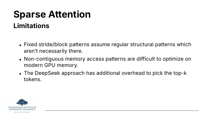
Three complaints about the sparse family. Read them as three different failure modes.

The idea behind each

Structural mismatch. Strided and block patterns assume the interesting relationships in the sequence happen at fixed offsets. In images that is (roughly) true; in prose, not always. A sparse pattern that's wrong for your task simply hides the tokens you needed.
GPU-unfriendly memory access. Modern GPUs love coalesced reads: long, contiguous stretches of memory. A mask that says "grab keys 3, 47, 512, 5013" turns every attention step into a scatter/gather pattern that is much slower than its FLOP count would suggest.
Selection overhead. DeepSeek's dynamic mask is not free. You pay for the low-precision indexing head and for the top-k sort. If k is small enough this pays back, but the crossover point is real.

⚠ Watch out

People quote FLOPs for sparse attention and it looks like a huge win. Then they benchmark on an actual GPU and the wall-clock is only marginally better. The second bullet is why. On A100/H100 hardware, contiguous memory access matters as much as arithmetic count.

§4Hybrid attention: BigBird's three-in-one mask

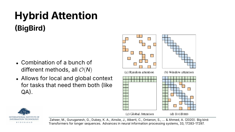
BigBird (Zaheer et al., 2020) is the answer to a natural question: if sliding is good for local context and a few global tokens are good for propagating summary information, why not stack both, and sprinkle in a bit of randomness for good measure? The three components combine into a mask that is still $O (n)$ but that provably approximates full attention.

Slide 11 / 21

Hybrid Attention (BigBird): combination of methods, all O(N). Allows local and global context for tasks that need both (like QA). Four attention masks: random, window, global, BigBird (all three combined).

slide 11 · BigBird = window + global + random

On the slide

The three building blocks and their combination:

(a) Random attention. Each query attends to r random past positions.
(b) Window attention. The familiar sliding band.
(c) Global attention. A small set of designated tokens that see everything and are seen by everything (the L-shaped green frame).
(d) BigBird. All three composed into one mask.

What to take from it

Each pattern is $O (n)$ on its own; their union is still $O (n)$ . The window gives you the local structure that words in a sentence share; the global tokens give you the CLS/question hub through which any two positions can reach each other in two hops; the random links give the graph the small-world property that makes the whole thing a good approximation to full attention. The paper proves BigBird is a universal approximator of sequence functions and is Turing complete, both properties that full attention has too.

✦ Key takeaway

The random links look wrong at first. Why would you attend to a random token? The reason is graph-theoretic. In a small-world graph, a handful of long random edges collapses the diameter of the graph from "long" to O(log n). That means information can flow between any two tokens in a few hops even without a global hub.

Slide 12 / 21

Hybrid memory table: g=64 global, w=128 window, r=64 random. KV cache is (g+w+r)·l·2·d_h = 0.06 MParams / 4 MB.

slide 12 · BigBird memory table

On the slide

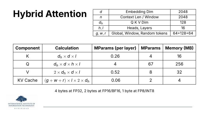
Reference model again, with the row that identifies the three budgets: g = 64 globals, w = 128 window, r = 64 randoms. KV cache is now $(g + w + r) \cdot l \cdot 2 \cdot d_{h}$ , a slightly bigger budget than plain sliding, but still constant in n.

Why the cache doesn't blow up

Because every one of g, w, r is a small fixed number, their sum is a small fixed number. Doubling the sequence length doesn't change any of them. That is exactly the property you buy with any of the sparse families.

Slide 13 / 21

Hybrid Attention Limitations: which tokens count as global is task-dependent; combining sliding, random, global patterns makes parallelisation tricky.

slide 13 · BigBird limitations

On the slide

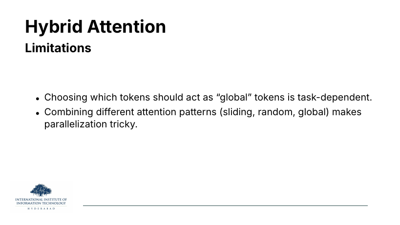
Two honest problems with BigBird.

The idea behind each

First, global tokens are task-dependent. For a QA task the question tokens are natural globals. For a coding task, maybe the function signature. For plain generation, there's no obvious answer, and picking the wrong ones wastes the strongest slot in your mask.

Second, parallelisation is fiddly. Windowed attention on its own is a clean band-matrix operation the GPU loves. Add scattered globals and random links and you get exactly the non-contiguous memory access problem from slide 10: mask kernels get complicated, and squeezing the last 2× out of them requires the kind of custom CUDA that few teams write.

§5Linear attention: rewrite the algebra

Everything up to here has been a game with masks: skip cells, rearrange them, choose them, but still compute the surviving cells the standard way. Linear attention gives up on the mask altogether and attacks the shape of the equation itself. Katharopoulos et al. (2020) noticed that if the softmax is replaced with a factorable kernel, the associativity of matrix multiplication lets you rearrange the product so the n-by-n matrix never appears.

Slide 14 / 21

Linear Attention: standard attention is O(N^2) because softmax(QK^T/sqrt(d_k)) is N×N. The exponentiation in softmax can be replaced by a similarity function, e.g. a kernel map phi. Applying phi is O(N d_k) because the kernel can be a recurrent computation.

slide 14 · four-bullet setup

On the slide

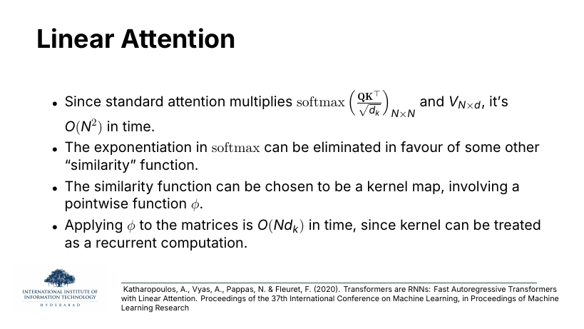
The pitch, in four bullets:

Standard attention builds an N×N matrix, so it costs O(N²) time.
The exponential inside softmax is the villain: it couples every q_i to every k_j nonlinearly, so the sum cannot be factored.
Replace exp with a factorable kernel written as $φ (q) \cdot φ (k)$ for some feature map φ.
Then the whole thing can be reorganised as a recurrence, giving $O (N d_{k})$ , linear in the sequence length.

Why softmax is the obstacle

Softmax attention computes $o_{i} = \frac{\sum_{j} exp (q_{i}^{⊤} k_{j}) v_{j}}{\sum_{j} exp (q_{i}^{⊤} k_{j})}$ . The exp knots q_i and k_j together, so you cannot pull q_i out of the sum. Replace exp by a bilinear form and suddenly you can.

Slide 15 / 21

Standard softmax attention: o_i = sum_j exp(q_i^T k_j) v_j / sum_j exp(q_i^T k_j). The exponential couples q and k inside the nonlinearity; must materialise the n×n QK^T; cost O(n^2 d) time, O(n^2) memory.

slide 15 · softmax attention, restated

On the slide

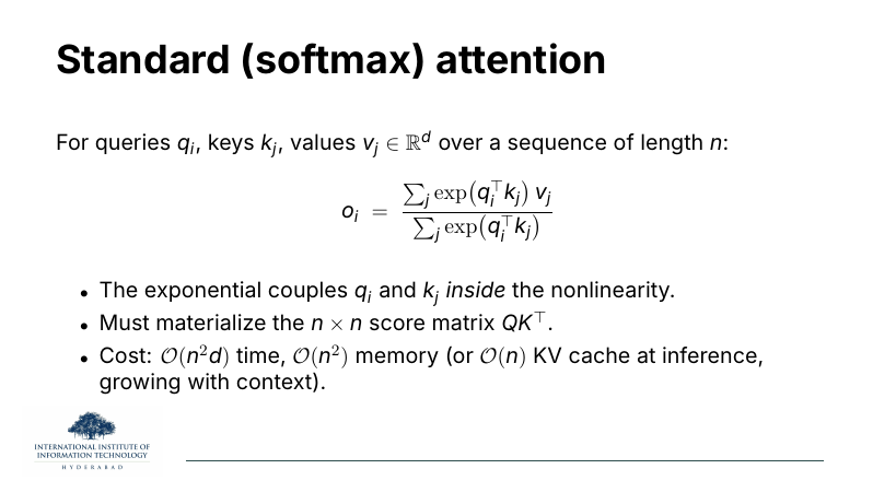
The exact softmax attention formula for a single query q_i, plus a three-bullet postmortem. exp couples q and k inside the nonlinearity, so the n×n score matrix $Q K^{⊤}$ has to be materialised. Cost is $O (n^{2} d)$ time and $O (n^{2})$ memory.

Why this restatement matters

Compare this to slide 16. Both compute an output that is a normalised weighted sum of values. The only difference is what plays the role of the "weight". This slide fixes what we are trying to escape.

Slide 16 / 21

The linearisation trick: replace exp(q^T k) with phi(q)^T phi(k). Then o_i = phi(q_i)^T sum_j phi(k_j) v_j^T / phi(q_i)^T sum_j phi(k_j) = phi(q_i)^T S / phi(q_i)^T z. S and z are independent of i — compute once, cost O(d'd) per query. Total O(n d' d), memory independent of n.

slide 16 · the linearisation trick

On the slide

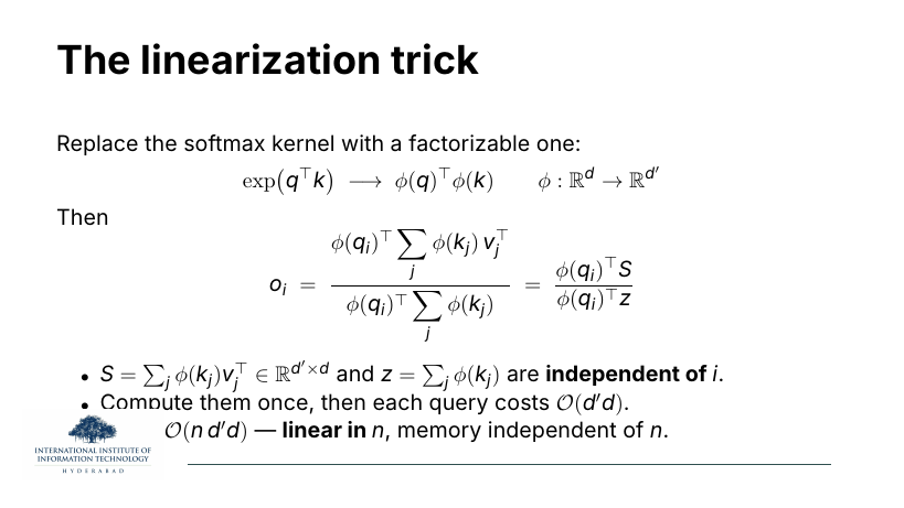
The one derivation you must remember from this lecture. Replace $exp (q^{⊤} k)$ with the factorised kernel $φ (q)^{⊤} φ (k)$ . Now the sum over j factors:

$o_{i} = \frac{φ (q_{i})^{⊤} S}{φ (q_{i})^{⊤} z}$ with $S = \sum_{j} φ (k_{j}) v_{j}^{⊤}$ , $z = \sum_{j} φ (k_{j})$ .

Under the hood

Both S and z are sums over j that do not depend on i. Compute them once, in one pass through the sequence, then every query is an O(d′d) contraction with the same S and z. Total: O(n d′d), and (this is the killer property) memory independent of n. The n-by-n matrix never appears anywhere.

Slide 17 / 21

$Causal case: linear attention is an RNN. S_t = S_{t-1} + phi(k_t) v_t^T; z_t = z_{t-1} + phi(k_t); o_t = phi(q_t)^T S_t / phi(q_t)^T z_t. Matrix-valued hidden state S_t in R^{d'×d}. O(1) time and memory per token at inference — no KV cache. Katharopoulos et al 2020: 'Transformers are RNNs.'$

slide 17 · causal case is an RNN

On the slide

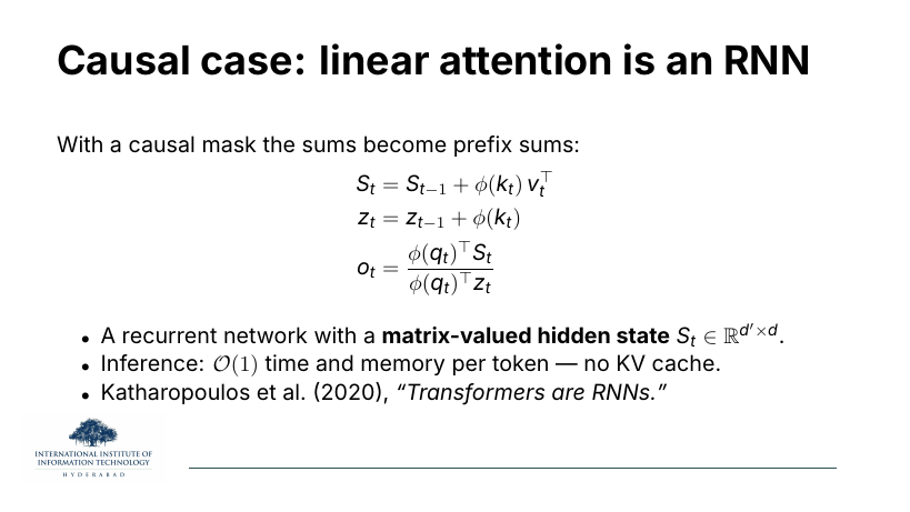
In the causal case, where token t may only attend to positions ≤ t, the sums that make up S and z become prefix sums. That means they can be maintained incrementally:

$S_{t} = S_{t - 1} + φ (k_{t}) v_{t}^{⊤}$

Why the RNN framing is deep

Look at that recurrence. It is a recurrent network: a hidden state $S_{t} \in ℝ^{d^{'} \times d}$ updated at each timestep by a rank-one addition. At inference, each new token costs O(1) time and memory, so no KV cache at all. That is why the paper is called "Transformers are RNNs". The transformer/RNN divide is smaller than you think; linear attention sits exactly on the seam.

Slide 18 / 21

Choosing the feature map phi. Table: elu(x)+1 (original, cheap, positive); positive random features (Performer, unbiased estimate of exp(q^T k)); identity/ReLU/SiLU (common in recent models); drop the denominator (replace with LayerNorm/RMSNorm output).

slide 18 · picking φ

On the slide

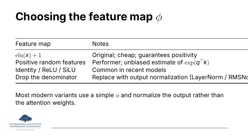
Four common choices for the feature map φ, each of which trades approximation quality for cost:

elu(x) + 1. The original Katharopoulos choice; guaranteed positive so the denominator never vanishes.
Positive random features. Performer (Choromanski et al., 2021); a randomised φ whose expectation exactly equals softmax, so you get an unbiased approximation of full attention.
Identity, ReLU, SiLU. Pointwise nonlinearities used in recent models. Cheap; empirically fine when combined with output normalisation.
Drop the denominator. Skip the z_t normaliser and let a LayerNorm on the output do the stabilising instead.

Why the choice matters

The kernel is the whole story. It decides how faithfully your linear attention imitates softmax, whether the denominator behaves numerically, and how stable training is. Modern models tend to pick a simple φ and rely on normalisation, rather than chase a fancy approximation of exp.

Slide 19 / 21

Why plain linear attention underperforms softmax. Bounded state: S_t is d'×d, fixed capacity regardless of context; retrieval of arbitrary past tokens degrades. Attention dilution: softmax gives near one-hot; kernel attention is smooth. No forgetting: S_t only accumulates, so interfering keys blend values.

slide 19 · why linear underperforms softmax

On the slide

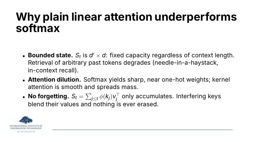
Three linked reasons that plain linear attention loses accuracy to softmax on long-context and retrieval-heavy tasks.

The idea behind each

Bounded state. The hidden state $S_{t}$ is d′×d. That's fixed. Softmax attention with a growing KV cache can always store one more exact key-value pair; linear attention overwrites. That is exactly why RNN models are bad at needle-in-a-haystack tests: the state can only carry so much.
Attention dilution. Softmax is a sharpener: because of the exp, it produces near one-hot weights when one key dominates. Kernel-based similarities are much smoother, so mass spreads across many keys and the "selection" behaviour that softmax gives you for free is weakened.
No forgetting. The recurrence $S_{t} = S_{t - 1} + φ (k_{t}) v_{t}^{⊤}$ only ever adds. Two keys with similar φ mash their values together in S, and nothing erases them. Later variants (Mamba, gated linear attention) add a forget gate to fix exactly this.

→ Keep reading

Every one of these limitations is the motivation for a later architecture. Bounded state and no forgetting are what State Space Models (Mamba) try to solve with data-dependent transition matrices. Attention dilution is what hybrid models like Jamba address by keeping some real softmax layers alongside linear ones.

Slide 20 / 21

Linear Attention memory: no context length parameter; Recurrent state (d_h^2 + d_h)·l = 0.03 MParams / 2 MB. Same K, Q, V as before.

slide 20 · linear memory (no n)

On the slide

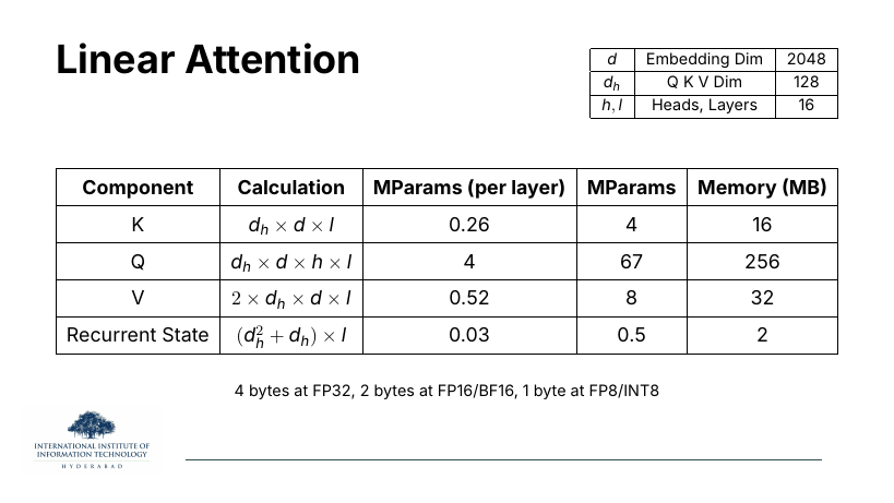
The reference table one last time. Notice what's missing from the parameter list at the top right: there is no n. Context length no longer appears in the memory budget, because the state doesn't depend on it.

The KV-cache row is renamed Recurrent State and computed as $(d_{h}^{2} + d_{h}) \cdot l$ . The $d_{h}^{2}$ comes from S_t being a d_h×d_h matrix (per layer); the extra d_h is the normalising vector z_t.

Why the row change is the whole story

Look at slide 5 (sliding), 9 (DeepSeek sparse), 12 (BigBird), 20 (linear) side by side. The parameter tables are almost identical. What changes across the four is exactly the last row, the running state. Sliding trims it to w; DeepSeek to k; BigBird to g+w+r; linear replaces it entirely with a fixed matrix. That's the story of the lecture in one row.

Slide 21 / 21

Linear Attention Limitations: sacrifices performance for efficiency; fixed-size recurrent state makes information retention harder; training unstable due to lack of softmax normalisation.

slide 21 · linear limitations

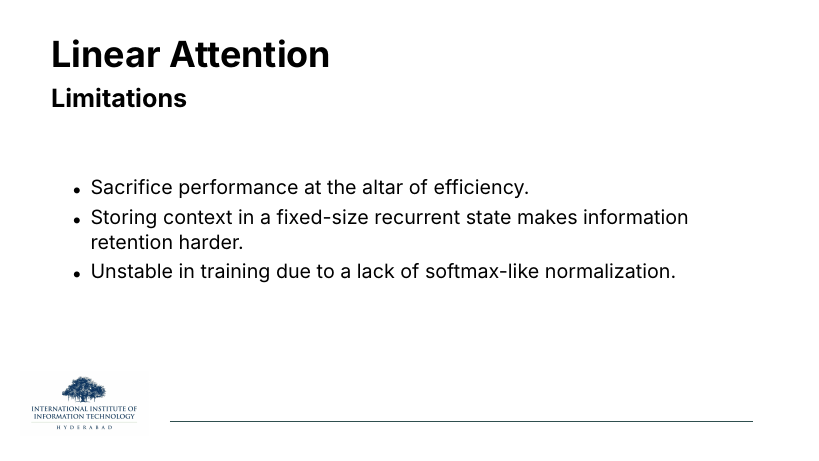
On the slide

The last slide of the lecture. Three honest bullets on why plain linear attention has not (yet) replaced softmax attention in production language models.

The idea behind each

The first bullet, "performance at the altar of efficiency", is the summary of slide 19. On benchmarks, softmax models still win at long-context retrieval and needle-in-a-haystack, though the gap is closing.

The second is the bounded-state problem restated: everything the model knows about the past has to fit in d′×d numbers per layer.

The third is a training-time concern. Without the softmax denominator's normalisation, the running sums S_t and z_t can grow without bound, leading to numerical issues. Modern variants patch this with LayerNorm/RMSNorm on the output (see slide 18's last row), gating, or careful φ choices. You can't just drop softmax and hope for the best.

Zoom out one last time. The lecture surveyed two philosophies for beating O(n²): skip cells (sliding, sparse, BigBird) and refactor the equation (linear). Both work, both cost you something, and both are living research. The next radical step, dropping attention entirely and replacing it with a state-space recurrence you can train in parallel, is the topic of the alternate-architectures block later in the semester.