Lecture 07 · 17 slides · September 3, 2026

Normalization: flatten the landscape so the network can walk.

Deep networks train by gradient descent, and gradient descent is only fast when the loss surface is roughly round. Raw features rarely make it so. This lecture is the accumulated fix: normalize activations (BatchNorm, LayerNorm, RMSNorm), normalize weights (WeightNorm), add residual shortcuts so gradients survive depth, then decide where in a transformer block the normalization actually goes (Pre-LN, Post-LN, DeepNorm, HybridNorm).

Lecture 07 17 slides Manish Shrivastava · Aparajitha Allamraju

§0The deck at a glance

The lecture starts with a picture argument: a linear-regression loss landscape is a squashed ellipse before normalization and a circle after. Once that motivation lands, four normalizers get introduced in quick succession (BatchNorm, LayerNorm, RMSNorm, WeightNorm), each a different axis along which to compute mean and variance. The rest of the lecture puts normalization into the transformer block: residuals, then Pre-LN vs Post-LN, then two modern refinements (DeepNorm for very deep stacks, HybridNorm for mixing LN and RMSNorm in one block).

§1Why normalize? the shape of the loss surface

Slides 1–5 build one argument by picture. Take the simplest possible model, look at its loss landscape when the features are raw, look at it again after standardising the features, and see the difference. Then read the four-bullet summary of what normalization is supposed to buy you overall.

Slide 01 / 17

Title slide: Normalization, Advanced NLP M26, Manish Shrivastava + Aparajitha, IIIT Hyderabad, September 3 2026

slide 01 · title

On the slide

Lecture 7 of Advanced NLP Monsoon 2026. Co-taught by Manish Shrivastava and Aparajitha Allamraju. Normalization is a small word for a large family of tricks: any operation whose job is to keep activations, weights, or gradients in a numerical range where optimisation actually works.

What to take from it

Historically, deeper networks kept getting harder to train. Not because the loss got harder in principle, but because the numerical dynamics went bad: activations blew up or collapsed to zero, gradients vanished or exploded, learning rates that worked at layer 2 broke layer 20. Every idea in this lecture is a specific answer to a specific instance of that problem. Normalization is the reason transformers can be stacked 100 layers deep at all.

Slide 02 / 17

Setup: a parametric function y = a x_1 + b x_2 fit by minimising L = (1/m) sum_i (y_i − ŷ_i(a,b))^2.

slide 02 · the toy problem

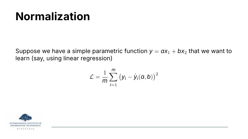
On the slide

Two-parameter linear regression: predict y from features x₁ and x₂ using weights a and b. Train by mean-squared error.

What to take from it

This is the smallest model that can still demonstrate the problem. Two parameters means the loss is a function of two numbers, which means we can literally plot the landscape on the next slide. Nothing about the argument depends on the model being simple — the same bad geometry appears in a transformer, just in a million-dimensional space you can't draw.

Slide 03 / 17

Contour plot of L(a,b): a very narrow vertical valley, elongated by roughly 20× along b relative to a.

slide 03 · the ellipse from hell

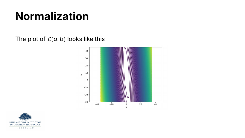
On the slide

The loss surface for that two-parameter regression when the two features have very different scales. It's an extremely elongated ellipse — a narrow trench that runs almost straight up and down in the (a, b) plane.

Why the picture is bad news

Gradient descent takes a step in the direction of steepest descent. On this landscape steepest descent points nearly perpendicular to the trench, not along it. The optimiser bounces from one wall to the other, making tiny net progress toward the minimum. To stay stable you have to shrink the learning rate, which makes progress along the long axis even slower. This is what people mean by a poorly conditioned optimisation problem.

Slide 04 / 17

After standardising features x_i ↦ (x_i − E[x_i]) / Var(x_i), the loss landscape becomes concentric circles centred near the origin.

slide 04 · standardise, and the ellipse becomes a circle

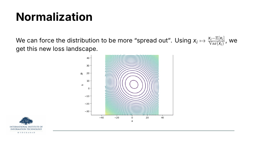
On the slide

The exact same regression problem, but with the features standardised: $x_{i} \mapsto \frac{x_{i} - 𝔼 [x_{i}]}{Var (x_{i})}$ . The contours become concentric circles — perfectly conditioned.

Why this is the whole idea

On circles, steepest descent points straight at the minimum. Any reasonable learning rate converges in a few steps. Nothing about the model changed; the input changed. Standardising features rescales the axes of the loss surface until they are the same length. That's it. Every normalisation scheme in this lecture is a more elaborate version of the same move, but applied to the activations inside the network rather than only the raw inputs.

✦ Key takeaway

Normalisation is a geometry fix. It doesn't change what the network can represent; it changes the shape of the loss surface into one that gradient descent can actually walk down.

Slide 05 / 17

Why normalization? Four bullets: increase speed of convergence; reduce sensitivity to input features; reduce overfitting; help generalization.

slide 05 · the four-bullet pitch

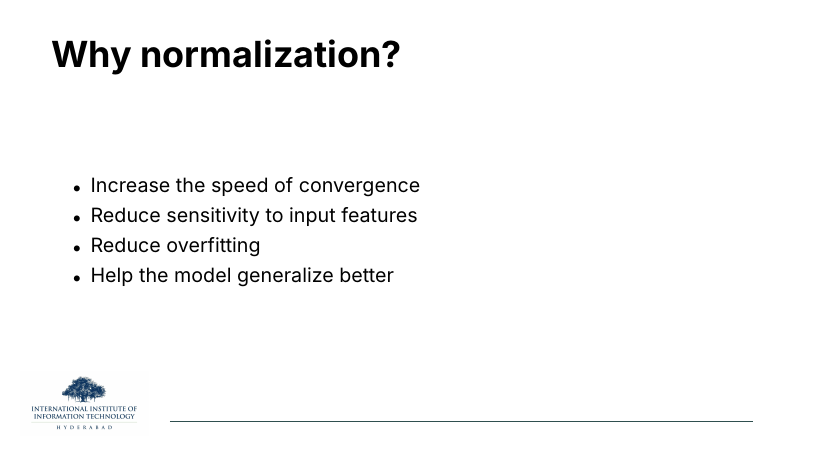
On the slide

Four benefits attributed to normalization: faster convergence, less sensitivity to feature scale, less overfitting, better generalisation.

What to take from it

The first two are the geometry story from slides 3–4. The last two are more subtle. Normalising a hidden layer means the units to the next layer always see a stable distribution — the network doesn't have to waste capacity re-learning how to handle a shifted scale every batch. That reduces the effective number of parameters that need tuning, which is one way to see the mild regularisation effect of BatchNorm and its relatives.

⚠ Watch out

"Reduces overfitting" is not the same as "replaces dropout". Normalization gives a small, incidental regularisation effect (BatchNorm gets it from batch statistics being noisy; LayerNorm gets almost none). Don't drop dropout or weight decay because you added normalization.

§2The four flavours: same equation, different axis

Slides 6–10 introduce four normalisers. The first three (BatchNorm, LayerNorm, RMSNorm) all have the same shape: subtract a mean, divide by a standard deviation, rescale and shift by learnable γ and β. The only thing that changes is which axis you take the statistics over. WeightNorm is the odd one out: it normalises the parameters, not the activations.

Slide 06 / 17

BatchNorm: normalizes across a batch of inputs index-wise. μ_i = (1/B) Σ_b x_i^(b); (σ_i)^2 = (1/B) Σ_b (x_i^(b) − μ_i)^2; y_i^(b) = γ_i (x_i^(b) − μ_i)/√((σ_i)^2 + ε) + β_i. Ioffe & Szegedy 2015.

slide 06 · BatchNorm (index-wise, across the batch)

On the slide

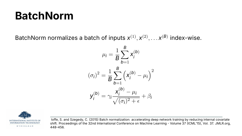
BatchNorm, from Ioffe & Szegedy (2015). For each feature index i, you take the mean and variance over the batch — that is, over all B examples that happen to be in the mini-batch — then standardise every sample using that per-feature statistic, then rescale by learnable $γ_{i}$ and shift by learnable $β_{i}$ .

Why "index-wise"

Read it as: pick a feature (say the 5th neuron's output). Now look at that neuron's value across all B samples in the batch. That's a length-B vector. Standardise it. Do that independently for every neuron. So the statistics couple samples to each other but keep the features independent.

⚠ Watch out

The batch statistic is why BatchNorm has two failure modes that matter for NLP. First, small batches give noisy estimates of μ and σ — with batch size 1 you can't even compute a variance. Second, at inference you have to keep running-average estimates because there's no batch, and if those averages don't match the training distribution you silently underperform. Both problems are why NLP mostly moved to LayerNorm.

Slide 07 / 17

LayerNorm: normalizes input-wise. μ^(b) = (1/d) Σ_i x_i^(b); (σ^(b))^2 = (1/d) Σ_i (x_i^(b) − μ^(b))^2; y^(b) = γ^(b) (x^(b) − μ^(b))/√((σ^(b))^2 + ε) + β^(b). Ba, Kiros & Hinton 2016.

slide 07 · LayerNorm (input-wise, across features)

On the slide

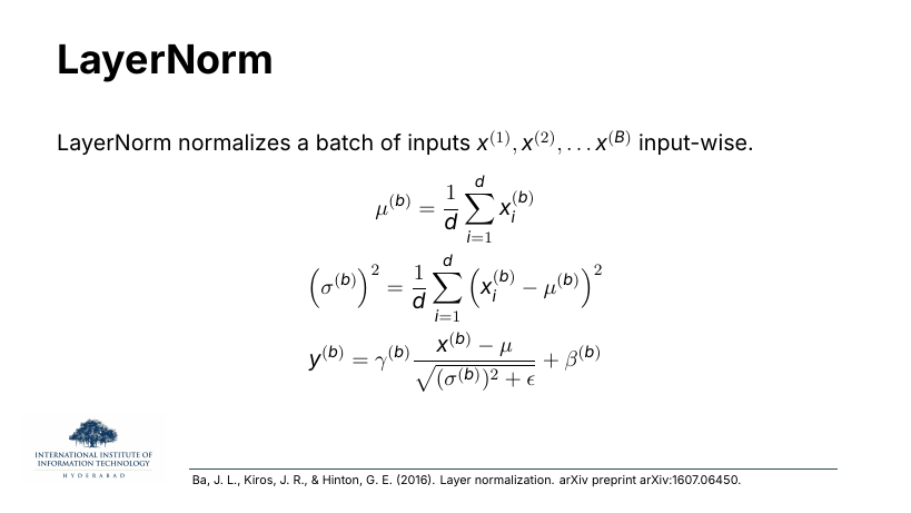
LayerNorm, from Ba, Kiros & Hinton (2016). Same three-step recipe as BatchNorm, but the mean and variance are taken per sample, over its feature dimensions. So the sum runs over i = 1…d, not over the batch. Every sample carries its own $μ^{(} b)$ and $σ^{(} b)$ .

Why LayerNorm wins for transformers

Every one of BatchNorm's failure modes disappears. Batch size doesn't matter — the statistic is computed inside one sample. Variable-length sequences don't matter — again the statistic is per-token. Training and inference behave the same because there's no running average to maintain. That's why every big language model uses LayerNorm (or one of its cousins), not BatchNorm.

Under the hood

In transformers the "sample" is usually one token: for each token position, you look at its d-dimensional embedding, standardise those d numbers among themselves, then apply per-feature γ and β. Two tokens in the same sequence are normalised independently.

Slide 08 / 17

Two 3D cubes with axes (Sentence Length, Feature, Batch Dimension). LayerNorm highlights a slice along the feature axis at one batch position; Batch/Power Normalization highlights the full sentence-length × batch face at one feature position.

slide 08 · which axis do you normalise over?

On the slide

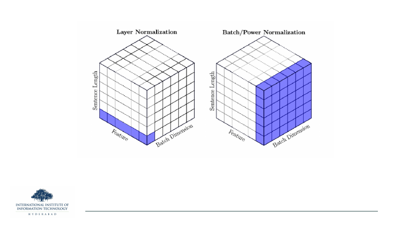
The clearest picture of the difference. The activation tensor has three axes: batch, sentence length, and features. LayerNorm slices along the feature axis (blue face on the left), pooling per token. BatchNorm (and PowerNorm) slices along the batch + sentence plane (blue face on the right), pooling per feature.

What to take from it

Everything else — GroupNorm, InstanceNorm, RMSNorm — is just a different choice of face on this cube. Once you can read the picture, you can tell which normalizer any paper is proposing by which face they colour in. That's the single most useful mental model in this section.

Slide 09 / 17

RMSNorm: LayerNorm with μ=0 enforced. y^(b) = γ^(b) x^(b) / √((1/d) Σ_i (x_i^(b))^2) + β^(b).

slide 09 · RMSNorm (LayerNorm minus the mean)

On the slide

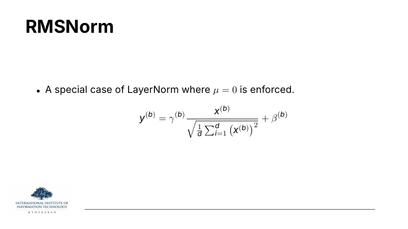
RMSNorm. LayerNorm normally does two things: recenter (subtract the mean) and rescale (divide by the standard deviation). RMSNorm drops the recentering step and only rescales, using the root-mean-square of the activations directly.

Why give up the mean subtraction

Empirically the recentering step contributes almost nothing to the quality of the model but costs a pass through the data to compute μ. Dropping it saves ~20% of the normaliser's compute and shows no measurable quality regression. That's why big open-source LLMs (LLaMA, Mistral, Gemma, Qwen) all switched to RMSNorm. Papers by Zhang & Sennrich (2019) first proposed it; wide adoption came four years later.

✦ Key takeaway

RMSNorm = LayerNorm with a compute discount. Same shape, same γ/β, one fewer statistic. If a paper says "we use RMSNorm", read it as "we use LayerNorm and don't care about the centring".

Slide 10 / 17

Weight Normalization: separate weight vectors into magnitude and direction. WeightNorm(x) = (g/||v||) v^T x + b. Applied per neuron. Salimans & Kingma 2016.

slide 10 · Weight Norm (normalise the weights, not the activations)

On the slide

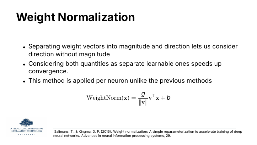
Weight Normalization, from Salimans & Kingma (2016). Instead of touching activations, decompose each neuron's weight vector into a direction (unit vector) and a learnable magnitude $g$ . Optimise the two separately.

Why the decomposition helps

Gradient descent updates weights by adding a scaled gradient. When direction and magnitude are entangled in one vector, an update that wanted to change only the length of v also nudges its direction, and vice versa. Separating them means the optimiser gets a cleaner set of "knobs" and can move the two independently. This speeds convergence in some settings.

⚠ Watch out

Unlike the other three, this one never caught on in transformers. It doesn't remove the ill-conditioning problem from activations at all — it only fixes weight geometry. Modern architectures either don't need it (because LayerNorm handles the harder problem) or fold something equivalent into the initialisation scheme.

§3Residual connections: let the gradient survive depth

Normalisation fixes the geometry of one layer. Residual connections fix the geometry between layers. Slide 11 gives the one-line formula that appears in every transformer block; slide 12 shows why, visually, deep networks without residuals are basically untrainable.

Slide 11 / 17

$Residual Connections: x_{L+1} = σ(x_L + F(x_L)). Used in the original transformers paper; well-known to mitigate vanishing gradient since the additive gradients dominate the multiplicative gradients.$

slide 11 · the residual formula

On the slide

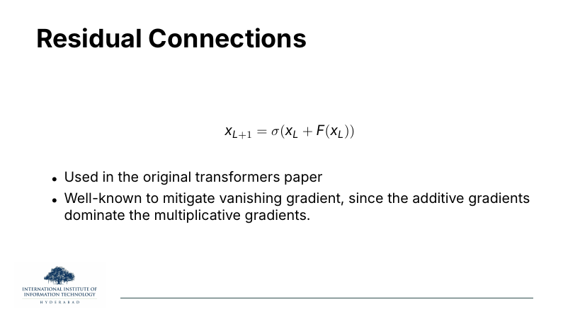
The one equation that made deep networks trainable. Layer L+1's output is not just F applied to layer L's input — it's the input plus what F computed on it (with a nonlinearity σ around the sum). Introduced by ResNet (He et al., 2015), used everywhere since.

Why residuals fix vanishing gradients

Backprop multiplies gradients through the chain of layers. If each layer's local Jacobian has singular values less than 1, the gradient shrinks exponentially with depth — that's the vanishing gradient problem. With a residual, the derivative of x_L+1 with respect to x_L gets an extra + I from the shortcut, so even if F's local Jacobian collapses to zero, the gradient still has a straight-through path of magnitude 1 back to earlier layers. Additive contributions dominate multiplicative decay.

Under the hood

Read $x_{L + 1} = x_{L} + F (x_{L})$ as "the next layer's job is to correct the previous representation, not replace it". A layer that can't help sets its F ≈ 0 and the identity flows through untouched. That means extra depth never hurts you: worst case, a redundant layer becomes a no-op.

Slide 12 / 17

ResNet-56 loss surfaces: without skip connections, a jagged mountain range full of local minima and cliffs; with skip connections, a smooth single basin. Li, Xu, Taylor, Studer & Goldstein 2018.

slide 12 · what depth looks like with and without residuals

On the slide

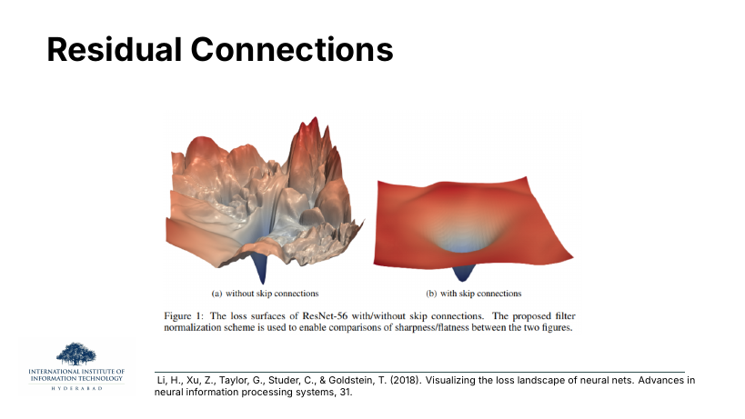
Two visualisations of the same 56-layer ResNet's loss landscape, from Li et al. (2018). On the left, the network trained without skip connections: a fractal-looking terrain of peaks and canyons. On the right, the same network with skips: a smooth bowl with a single obvious minimum.

What to take from it

This is the picture people mean when they say "residuals make deep networks trainable". The landscape on the left is what your optimiser sees, and it is essentially impossible to descend without landing in a local minimum or a saddle. The landscape on the right is what you get for free by adding an $x + \dots$ in every block.

✦ Key takeaway

Normalisation makes the local geometry inside each layer nicer. Residuals make the global geometry across layers nicer. Every transformer needs both.

§4Pre-LN vs Post-LN: where inside the block?

Once you have LayerNorm and residuals, you have a choice about where in the block the LayerNorm sits. Two placements dominate. The original transformer paper (Vaswani et al., 2017) put it after the addition (Post-LN). The community converged onto putting it before the sub-layer (Pre-LN) because it trains much more reliably. Both are still around, and they behave differently in specific ways.

Slide 13 / 17

Two transformer block diagrams. (a) Pre-LN: LayerNorm sits inside the residual branch, before Attention and before FFN, and the addition happens on the raw residual. (b) Post-LN: Attention and FFN feed into an addition with the residual, then LayerNorm sits after the addition. Xiong et al. 2020.

slide 13 · Pre-LN vs Post-LN, in a picture

On the slide

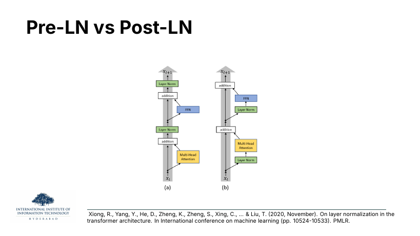
Two block diagrams from Xiong et al. (2020). Both are one layer of a transformer, both have Multi-Head Attention, an FFN, additions, and LayerNorm — the arrangement is what changes.

(a) Pre-LN: Norm → sub-layer → add. The LayerNorm is applied to the residual branch before it enters attention or the FFN. The addition is on raw x_L.
(b) Post-LN: sub-layer → add → Norm. Attention or FFN runs on x_L, its output is added to the residual, then LayerNorm runs on the sum. This is the original 2017 layout.

Why one-line difference, big effect

In Post-LN, the residual path itself gets scaled and shifted by LayerNorm at every layer. Small errors in that normalisation compound down the stack. In Pre-LN, the residual path is untouched — the identity connection runs unnormalised all the way from input to output, and LayerNorm only affects what gets added in. That's why Pre-LN behaves like a proper residual network and Post-LN doesn't quite.

Slide 14 / 17

Pre-LN vs Post-LN tradeoffs: Post-Norm makes training unstable and can lead to vanishing/exploding gradients; done carefully Post-Norm doesn't lose information; Pre-Norm stabilises training but leads to representation collapse (each layer represents nearly the same information, measured by cosine similarity).

slide 14 · the tradeoff nobody escapes

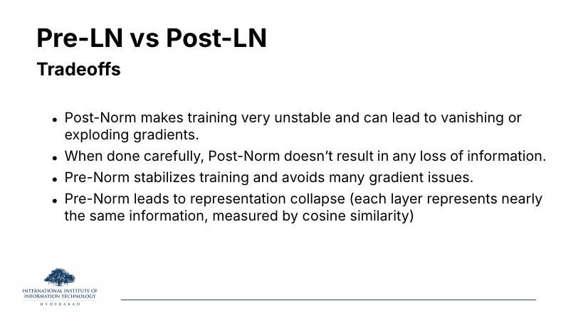
On the slide

Four bullets that summarise years of empirical work.

The idea behind each

Post-LN is unstable. Because the residual gets renormalised at every layer, gradient magnitudes at deeper layers can drift far from those at shallower ones. You often need warmup schedules and careful learning rates to train a Post-LN transformer at all.
Done carefully, Post-LN doesn't lose information. If you can get it to train, it tends to give slightly better final quality than Pre-LN. It's harder, not worse — nothing about the architecture caps its capacity.
Pre-LN stabilises training. The untouched residual pathway means gradients flow cleanly. You can use larger learning rates, skip warmup in some setups, and stack more layers.
Pre-LN causes representation collapse. This is the surprising finding. Because every layer's output is dominated by the (unchanged) residual, deep Pre-LN networks tend to have every intermediate layer looking similar to the next — measured by cosine similarity between layer outputs. You get depth without the diversity of representations depth is supposed to buy.

⚠ Watch out

The reflex "Pre-LN is just better" is not quite right. It's easier to train, which usually translates to better final numbers because you actually finish training. But if you have the budget and the patience for the tricks Post-LN needs, Post-LN gives you a real representation gain. This is why you still see Post-LN in some production models with careful engineering behind them.

§5DeepNorm: Post-LN that scales to 1000 layers

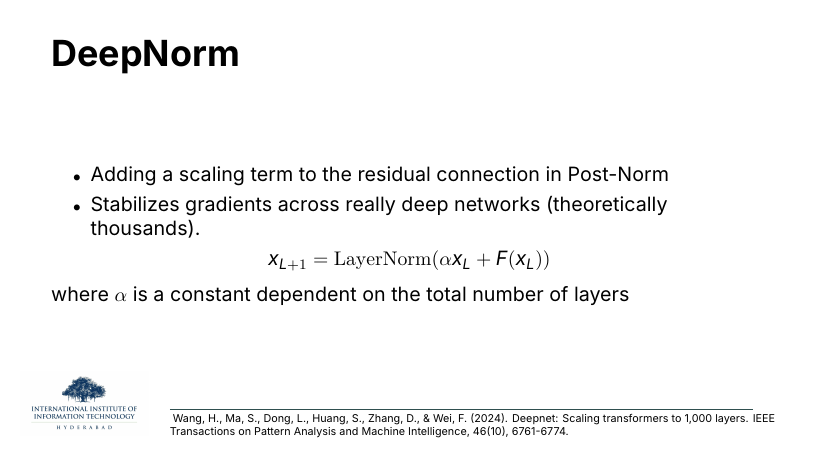
Slide 15 is a single equation that lets Post-LN work at extreme depth: multiply the residual by a constant α that depends on the total number of layers. That's it. Microsoft's DeepNet paper (Wang et al., 2024) uses this trick to stack transformers a thousand deep and still keep them stable.

Slide 15 / 17

$DeepNorm: add a scaling term α to the residual in Post-Norm; stabilises gradients across networks that are theoretically thousands of layers deep. x_{L+1} = LayerNorm(α x_L + F(x_L)), where α depends on the total number of layers. Wang et al. 2024.$

slide 15 · DeepNorm — one α buys 1000 layers of depth

On the slide

DeepNorm. Take the Post-LN block from slide 13(b), and multiply the residual by a constant α before the addition: $x_{L + 1} = LayerNorm (α x_{L} + F (x_{L}))$ . The α is a fixed constant chosen from the total number of layers.

Why one constant fixes it

The instability of Post-LN comes from the residual and the sub-layer output being on different scales after LayerNorm renormalises them repeatedly. α pre-weights the residual so that after all those renormalisations, its contribution stays comparable to the sub-layer's contribution. Wang et al. derive the exact α as a function of the depth (roughly $(2 N)^{1 / 4}$ for an N-layer encoder), so that gradient norms stay bounded regardless of depth.

✦ Key takeaway

DeepNorm is the whole reason people believe "you can train arbitrarily deep transformers". Before it, stacking beyond ~100 layers required either heroic tuning or Pre-LN's representation-collapse compromise. DeepNorm keeps Post-LN's quality with Pre-LN's trainability — for the price of one carefully chosen constant.

§6HybridNorm: use each normaliser where it earns its keep

The last two slides propose the newest twist. If RMSNorm is 20% cheaper than LayerNorm but slightly less numerically robust, and if some positions in the block are more sensitive to normalisation quality than others — why apply the same normaliser everywhere? HybridNorm (Zhuo et al., 2026) puts LayerNorm where it matters and RMSNorm everywhere else.

Slide 16 / 17

Four transformer block variants ×L: (a) Post-Norm — Norm placed at the top of each residual; (b) Pre-Norm — Norm inside each residual branch; (c) Pre-Norm with QK-Norm — separate Norms on Q and K inside attention; (d) HybridNorm — a combination that puts Norm in specific positions. Zhuo et al. 2026.

slide 16 · four transformer block layouts

On the slide

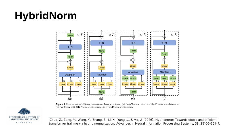
Four block designs, drawn as small diagrams to compare where the normalisers sit.

(a) Post-Norm: LayerNorm on the sum at the top of each block, as in the 2017 paper.
(b) Pre-Norm: LayerNorm inside the residual branch before attention and before FFN.
(c) Pre-Norm with QK-Norm: Pre-Norm, plus separate LayerNorms directly on the Q and K projections inside attention. Helps stabilise the softmax input scale.
(d) HybridNorm: puts LayerNorm at specific sensitive positions and RMSNorm at the rest, chosen empirically.

Why the picture, not just the equation

You cannot spot which normaliser is which from the maths — they all look identical on the page. Papers use these block diagrams because the placement is the whole contribution. Read them as circuit schematics: where the Norm box sits, and what its input is, determines what property the block gets.

Slide 17 / 17

HybridNorm intuition: post-attention normalization is (empirically) more sensitive to normalizer choice than other positions; using LayerNorm there and RMSNorm elsewhere gives meaningful speedup relative to LayerNorm-only without the catastrophic results likely when using only RMSNorm.

slide 17 · why the mix wins

On the slide

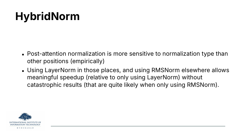
Two-bullet summary of why HybridNorm exists.

The idea behind each

Post-attention is the sensitive spot. Empirically, the LayerNorm that comes right after the attention output is the one where RMSNorm's shortcut hurts the most. Attention outputs can have skewed distributions that need proper mean-subtraction to stay tame.
Everywhere else is fair game. The remaining LayerNorms (before Q/K/V, after FFN) can be replaced by RMSNorm with negligible quality loss. You keep the speed win over an all-LayerNorm network while dodging the crashes you'd see in an all-RMSNorm network.

→ Trend to watch

This is the general shape of a lot of modern architecture research: not "invent a better normaliser" but "figure out where each one belongs". Similar arguments show up in FP8-training papers (some layers tolerate low precision, others don't) and in Mixture-of-Experts routing (some tokens want the big expert, others want the cheap one). Normalisation choice is now a per-position hyperparameter, not a global one.

Zoom out. Normalisation is layers of fixes for the same underlying disease: gradient descent hates poorly conditioned landscapes. Standardise inputs to fix the geometry within a layer (BatchNorm, LayerNorm, RMSNorm). Add residuals to fix the geometry across layers. Choose Pre-LN or Post-LN and live with the tradeoff. Scale to 1000 layers with DeepNorm. Mix normalisers per-position with HybridNorm. Every one of these is a small piece of geometry engineering, and each was worth a paper.