Seminar · Vishal Rao · 34 slides

Data Creation: a (very) high-level overview.

Every language model is a compressed summary of the data it saw. So the interesting question — the one this seminar takes seriously — is: where does that data come from, and who decides what makes the cut? Vishal walks the whole stack in one hour: scraping the open web (Common Crawl), curating it down to something a model can actually learn from (DCLM, FineWeb), synthesising new data when the well runs dry (WRAP, Self-Instruct, Evol-Instruct), the failure mode you get when models train on each other's output (model collapse), and the last stage almost nobody does honestly (benchmark decontamination).

Seminar 34 slides Vishal Rao

§0The deck at a glance

The seminar is organised as a survey rather than a deep dive on any one paper. Slide 2 lists 21 numbered topics; grouped, they fall into three big blocks. First, curation: how a raw web dump becomes a training set — Common Crawl → DCLM → FineWeb, with a subtractive pipeline that throws away ~98% of what it starts with. Second, synthesis: when curation isn't enough, use an LLM to write data — WRAP for pretraining, Self-Instruct and Evol-Instruct for post-training, then the failure mode (model collapse from Shumailov, and the accumulate-don't-replace fix from Gerstgrasser). Third, evaluation: benchmark decontamination as the honest but neglected step, plus a short note on faithfulness and diversity metrics. The tone throughout is "here's the survey shape of the field", not "here's the canonical answer".

§1What is data creation? and why bother.

Slides 1–4 set up the whole talk. The move from "find the data" to "create the data" is a deliberate one: it's what you do when scraping stops scaling, when the domain you care about doesn't have enough public text, or when licensing eats you alive. These slides also introduce the two words that will haunt the rest of the deck — faithfulness and diversity.

Slide 01 / 34

Title slide: Data Creation, A (VERY) high-level overview, over a stylised isometric illustration of servers and a robot stepping out of a phone.

slide 01 · title

On the slide

Title card. "Data Creation — A (VERY) high-level overview." The parenthetical is doing work: this deck is deliberately a survey pass, not a paper walk-through.

What to take from it

Data creation used to be a corner of NLP that only industrial labs cared about. In the last two years it's become the field's central bottleneck. Model architectures have largely stopped moving; what still moves benchmark numbers is the training set. So spend an hour with the shape of the space before you go deep on any one paper.

Slide 02 / 34

Seminar Structure: a 21-item numbered outline covering what is data creation, what makes good data, LLM-driven data generation, DataComp-LM, FineWeb, curation vs synthesis, terminology, the Pile, WRAP, Self-Instruct, Evol-Instruct, student-teacher paradigm, model collapse (Shumailov), Gerstgrasser's fix, evaluation, benchmark decontamination, LLM decontaminator, other evaluation methods, open problems, and bibliography.

slide 02 · seminar structure

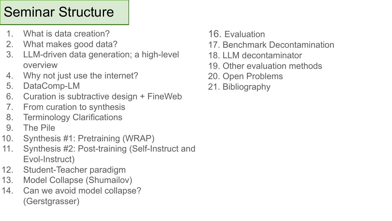
On the slide

Twenty-one bullets that map to the rest of the deck. Vishal grouped them roughly by pipeline stage: curation topics (4–6, 9), synthesis topics (7, 10–12), the model-collapse pair (13–14), and evaluation + decontamination (16–19). Open problems and the bibliography close it out.

What to take from it

The structure of the outline is the argument. Notice that curation and synthesis get almost equal airtime, and that evaluation gets its own third of the deck — a hint that the speaker thinks the evaluation half of the story is under-appreciated by everyone else.

Slide 03 / 34

What is Data Creation? Bullets: the field moves from finding data (scraping/licensing/begging) to deliberately designing and constructing data for downstream tasks. Long et al. reasons: data is expensive, scarce in the domains that matter most, legally constrained. Three-stage workflow — Generation, Curation, Evaluation (optional). Reference: Long et al., On LLMs-Driven Synthetic Data Generation, Curation, and Evaluation: A Survey.

slide 03 · what data creation actually means

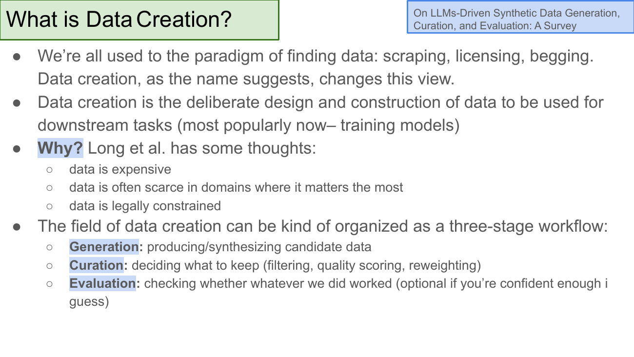
On the slide

The working definition: data creation is the deliberate design and construction of data for a downstream task. And a three-word taxonomy that will structure the rest of the deck: Generation → Curation → Evaluation.

What to take from it

The Long et al. survey identifies three pressures pushing labs to make their own data: cost, scarcity in high-value domains (medical, legal, low-resource languages), and legal constraints (copyright, GDPR, publisher lawsuits). Any one of these alone forces the shift; all three together explain why every serious lab now has a "data" team the same size as its "modelling" team.

✦ Key takeaway

The three-stage split is the mental model to hold onto for the rest of the seminar. Every paper Vishal covers is doing one (or two) of Generation, Curation, Evaluation. If you know which stage a paper is aiming at, you already know 60% of what it does.

Slide 04 / 34

What Makes Good (Generated) Data? Beyond cleanliness, spanning the necessary space, sufficient quantity, and being economical to generate, two requirements stand out: (1) Faithfulness — data must be logically and grammatically coherent; hallucination and the fat-tailed knowledge distribution of LLMs introduce noise. (2) Diversity — variation in generated data; hard because we can't estimate the underlying data-generating distribution, and LLMs' inherent biases lead to monotonic outputs even at high temperature. Reference: Gandhi et al., Better Synthetic Data by Retrieving and Transforming Existing Datasets, CMU.

slide 04 · what makes generated data actually good

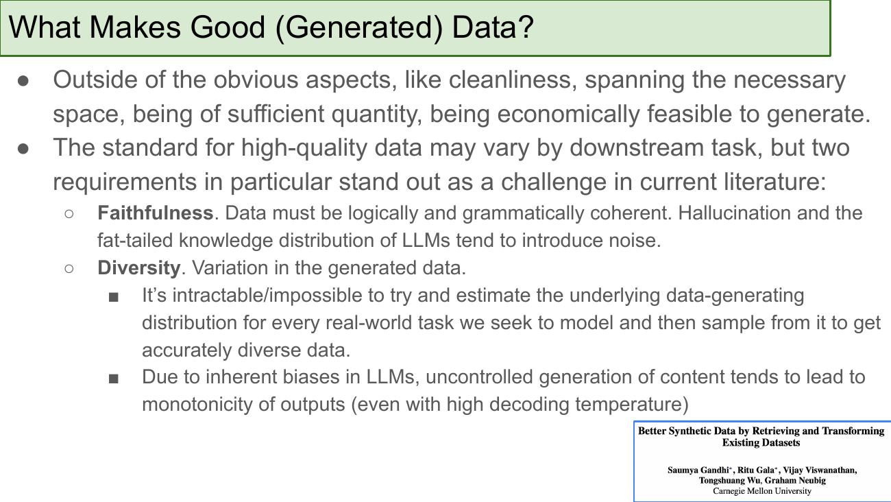
On the slide

Two quality axes that dominate the current literature on synthetic data. Faithfulness — is the data true, both logically and grammatically? And Diversity — does it span the space, or does the model keep writing the same essay?

Why these two, specifically

Faithfulness is threatened by hallucination and by the fat-tailed knowledge distribution of the generator — an LLM confidently emitting incorrect facts pollutes the training set. Diversity is threatened by the LLM's own biases: sample the same model a thousand times and you'll see the same handful of essay openings, the same three "helpful assistant" phrasings. Even cranking temperature up doesn't fix this — the mode-collapse is baked into the pretraining. The rest of the deck can be read as "here's how each pipeline stage tries to defend these two properties".

⚠ Watch out

Faithfulness and diversity trade off against each other. Filter hard for correctness (faithfulness up) and you tend to keep only the model's most-confident, most-generic outputs (diversity down). Every curation pipeline you'll see is basically a knob for setting that trade-off.

§2The three-stage pipeline: generation, curation, evaluation.

Slide 5 is the survey figure Vishal keeps returning to. It's worth reading carefully because everything that follows fits somewhere on this diagram.

Slide 05 / 34

LLM-Driven Data Generation, A High-Level Overview. Left: a stylised tree with clinical trials, healthcare analytics and table analysis as fruits, fed by synthetic data as nutrients. Middle: a pipeline diagram where a pretrained LM prompted with p on task T and seed data D_sup produces generated dataset D_gen; the formalism D_gen ← M_p(T, D_sup) and p(T, D) ← E(e_task, e_condition, e_demo) is shown. Right: a full taxonomy tree with three branches — I Generation (prompt engineering, multi-step generation), II Curation (sample filtering, label enhancement), III Evaluation (direct: faithfulness & diversity; indirect: benchmark & open).

slide 05 · the full taxonomy in one figure

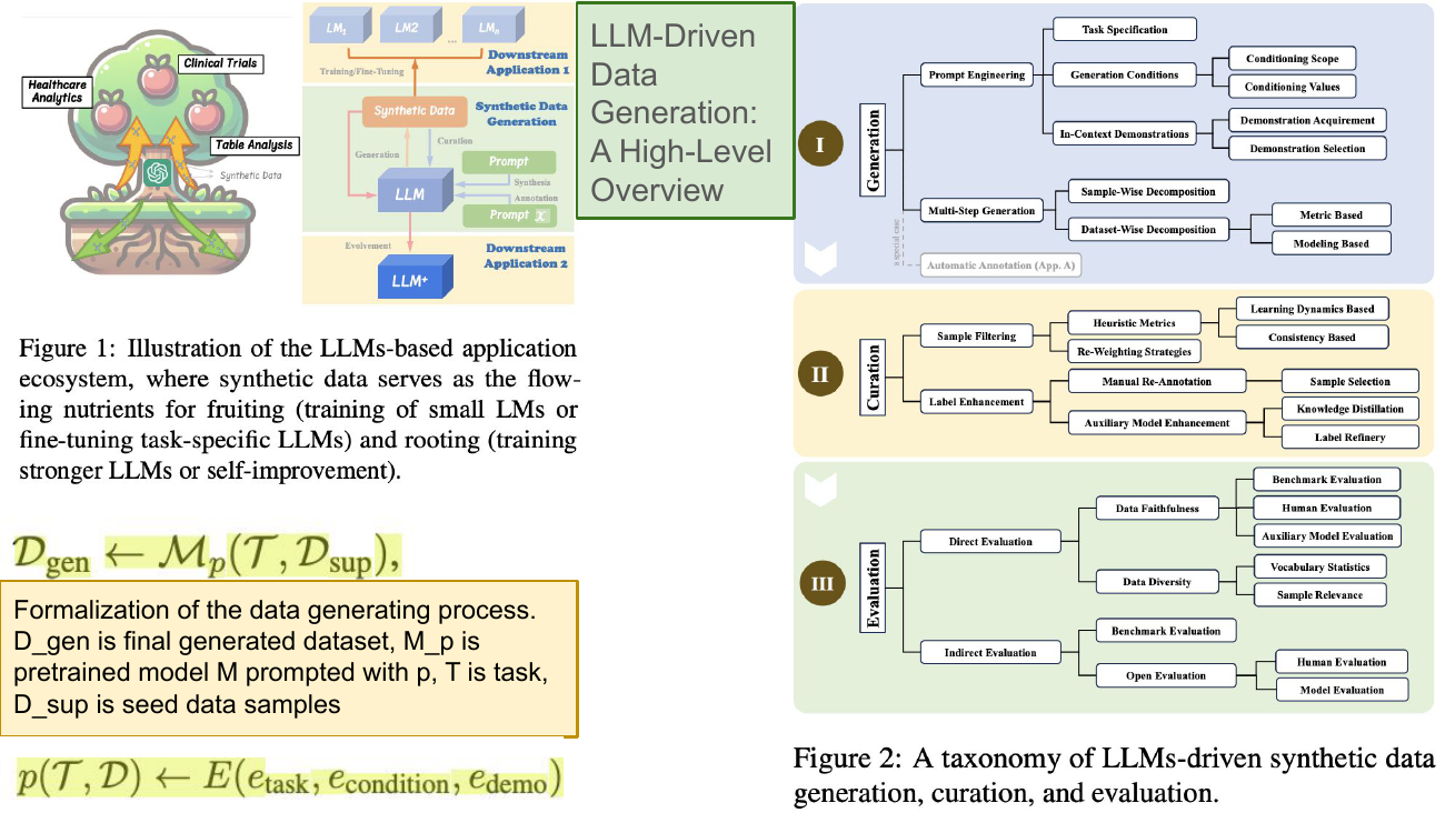
On the slide

Three panels from the Long et al. survey. The tree on the left is the metaphor — synthetic data feeds downstream applications like nutrients feed fruit. The pipeline in the middle is the formalism: a generator model $ℳ_{p}$ takes a task $𝒯$ and a seed $𝒟_{sup}$ and returns a generated dataset $𝒟_{gen}$ . The taxonomy on the right is the map.

What to take from it

Read the right-hand tree as a menu. When you meet a new "synthetic data" paper, you can usually place it at one leaf: is it fiddling with prompt engineering (task specification, generation conditions, in-context demonstrations)? Is it doing multi-step generation to decompose a hard task? Is it curation via heuristic filters or model-based re-weighting? Is it evaluation via faithfulness scoring or diversity statistics? The whole seminar is examples plucked from this tree.

→ Reference

Long, Wang, Xiao, Zhao, Ding, Chen & Wang, On LLMs-Driven Synthetic Data Generation, Curation, and Evaluation: A Survey (ACL Findings 2024, arXiv:2406.15126). This is the paper whose figure the whole deck's outline follows.

§3Curation: DCLM, FineWeb, and the 98% you throw away.

Slides 6–11 walk through curation from the top: Common Crawl, DataComp-LM (DCLM), the FineWeb pipeline, and MinHash as the workhorse deduplication trick. The provocation on slide 6 — why generate when you can use what already exists? — is worth taking seriously. For pretraining-scale data, curation is still the default, and it's a very specific kind of engineering: you build a waterfall of filters, and you measure success by how much of the input pool gets rejected.

Slide 06 / 34

Section divider slide: Curation — Why generate data when you can use what already exists?

slide 06 · section divider — Curation

On the slide

Section header for the curation block. The subtitle is a fair provocation: before you commit to writing synthetic data, ask whether cleaning what's already on the internet would be cheaper.

What to take from it

For pretraining scale (trillions of tokens), the answer is almost always "yes, use the web first". Synthesis is the tool you reach for when you've exhausted curation, or when the domain is one the web doesn't cover.

Slide 07 / 34

slide 07 · Common Crawl and why we all owe it a lot

On the slide

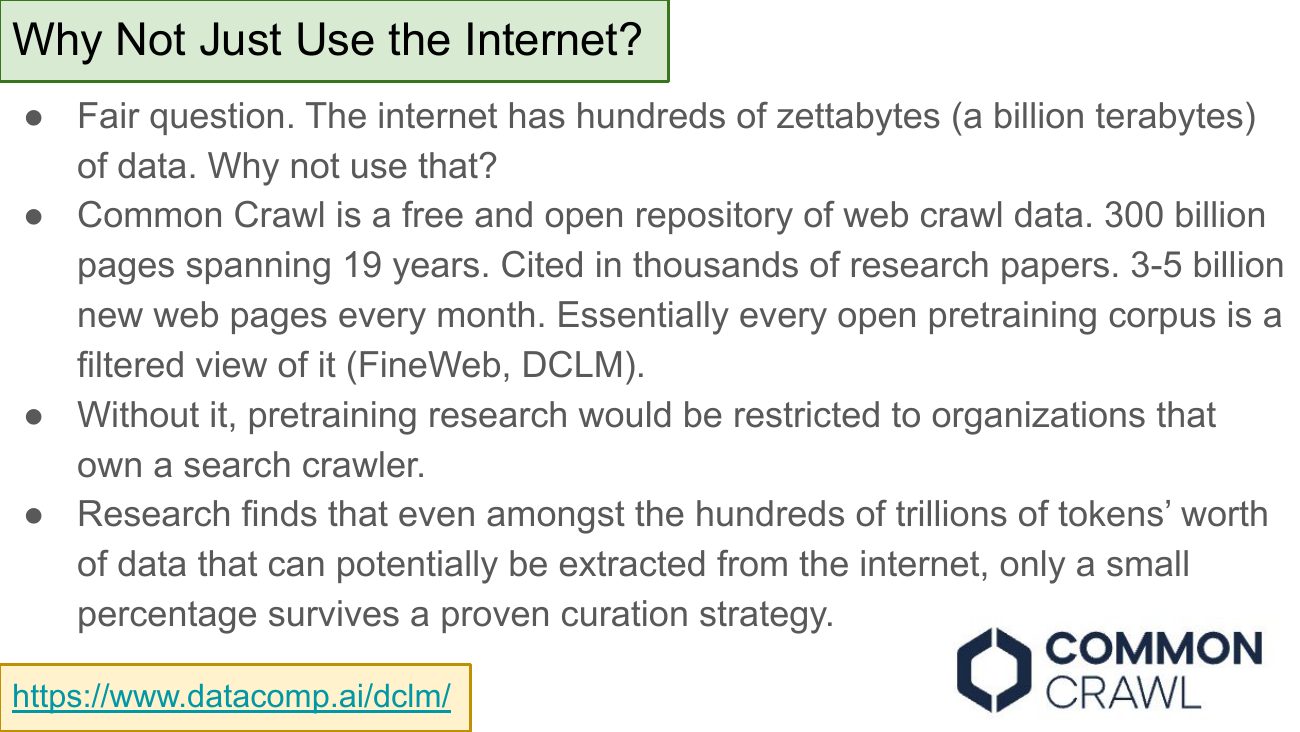
Common Crawl in numbers: 300B pages over 19 years, 3–5B new pages a month, free and open, cited in thousands of papers. Almost every open pretraining corpus you've heard of is a filtered view of it.

Why this matters more than it looks

Without Common Crawl, only companies that operate their own search engine (Google, Microsoft) could do pretraining research at scale — everyone else would be locked out. Common Crawl is the reason academic labs and open-source projects can even attempt to train frontier models. But — and this is the punchline of the slide — even from that mountain, only a few percent of tokens survive any serious curation pipeline. Raw web is mostly noise.

✦ Key takeaway

The public web is huge, but the trainable public web is small. Curation is the step that converts the first into the second.

Slide 08 / 34

DataComp-LM (DCLM): The Internet Data Curation Attempt. A Sankey diagram shows DCLM-Pool from Common Crawl (100%) shrinking through URL filter (0.8%), English filter (50.8%), other filters like word length and ellipsis count (9%), page length filter (7.9%), repetition filter (9.6%), word removal ratio filter (2%), heuristic cleaning (RefinedWeb reproduction) leaving 19.9%. Then deduplication (Bloom filter dedup) brings it to 13.7%, then FastText model-based filtering brings the final DCLM-Baseline to 1.4%. Body text: DCLM is a testbed for controlled dataset experiments aimed at improving LLMs. Starting corpus is 240T Common Crawl tokens (DCLM-Pool); after filtering the baseline training set is around 3.8T tokens. Roughly 98% of the pool is discarded before the model ever sees it. Reference: DataComp-LM: In Search of the Next Generation of Training Sets for Language Models.

slide 08 · DCLM as the reference curation waterfall

On the slide

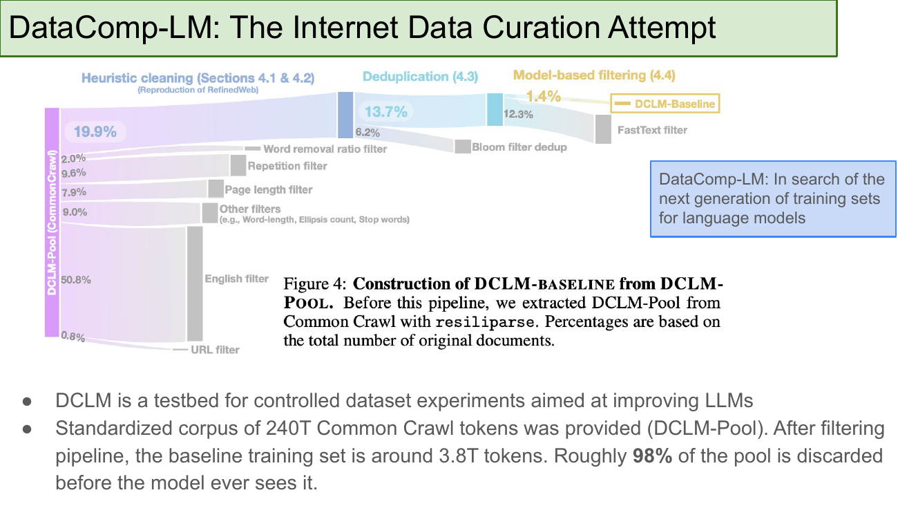
The Sankey diagram is the whole pipeline: 240T tokens of raw Common Crawl (DCLM-Pool) → URL filter → English filter → heuristic cleaning (page length, repetition, word-length, ellipsis, stop words) → deduplication → model-based filtering (FastText classifier) → 3.8T-token DCLM-Baseline.

Why the 98% discard is the story

Read the widths in the Sankey. At every stage the pipeline throws out most of what enters it, and the cumulative effect is that fewer than 2% of the original tokens make it into training. This is not a bug — the whole game is figuring out which 2%. DCLM's contribution is standardising the pool, the training recipe, and the 53-benchmark evaluation harness so that different filtering strategies can be compared apples-to-apples.

Under the hood

DCLM freezes everything except the filtering choice. You submit a filtering strategy, DCLM applies it, trains a model with a fixed recipe at a fixed scale, and reports the downstream scores. The point is that the leaderboard is comparing data, not modelling tricks.

Slide 09 / 34

Four-step DCLM workflow diagram. A: Select a scale (400M-1x, 1B-1x, 3B-1x, 7B-1x, or 7B-2x). B: Build a dataset — either filter DCLM-Pool (filtering track) or mix in external data (mixing track). C: Train a language model with a fixed recipe. D: Evaluate on 53 downstream zero-shot and few-shot tasks. Side note explains MMLU: Massive Multitask Language Understanding, a 57-subject academic test. Bottom table compares FineWeb edu vs DCLM-BASELINE at 7B/0.14T and 0.28T on Core, MMLU, Extended benchmarks: DCLM-BASELINE beats FineWeb edu at every scale, and DCLM-BASELINE + StarCoder + ProofPile2 at 7B/2.6T scores 57.1 / 63.7 / 45.4.

slide 09 · DCLM workflow + head-to-head numbers

On the slide

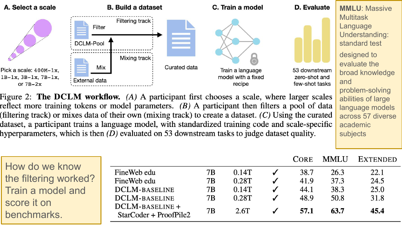
The full DCLM protocol drawn as four boxes (A: pick a scale; B: build the dataset via filtering or mixing; C: train the model with a fixed recipe; D: evaluate on 53 tasks) and the leaderboard-style table underneath.

What to take from it

Two things. First, the DCLM answer to the "how do we know curation worked?" question is train a model and score it. That's expensive but honest. Second, look at the table: DCLM-Baseline beats FineWeb-edu at every matched scale, and by non-trivial margins on MMLU (50.8 vs 37.3 at 0.28T tokens). The right curation strategy is worth more than an order of magnitude of extra training tokens.

Slide 10 / 34

Curation is Subtractive Design. What does that 98% discarding procedure actually look like? A pipeline diagram: Text extraction → Language ID → Heuristic filters → PII removal → MinHash dedup → Benchmark decontamination (highlighted in purple) → Model-based quality scoring. Each step has a note: WARC files parsed with trafilatura; classifier + URL blocklist for English confidence; rules from comparing high vs low quality stats (e.g. terminal punctuation ratio); regex scrubbing of emails and IPs; deduplication that is not monotone with quality; removing training documents that contain evaluation items; Llama-3-70B-Instruct annotates documents for educational value 0-5. Reference: The FineWeb Datasets: Decanting the Web for the Finest Text Data at Scale.

slide 10 · the FineWeb pipeline, step by step

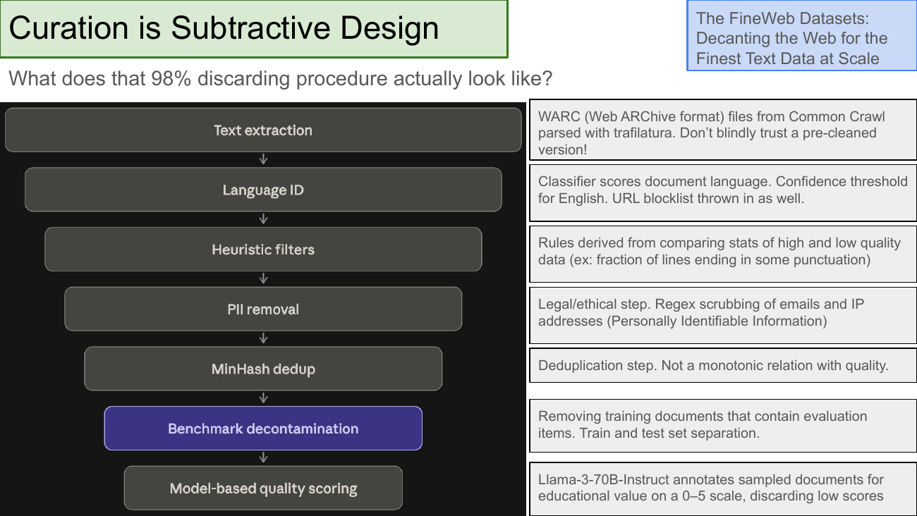
On the slide

The FineWeb pipeline as a vertical stack of seven filters. Each has a one-line rationale on the right. The one drawn in purple — benchmark decontamination — is the step that will come back to haunt the evaluation section.

Why "subtractive design" is the right framing

Compare this to how you'd build a website or a network. There, engineering is additive: you write components, glue them together, add features. In data curation, every step is a filter that removes documents. The dataset you ship is the hole in the negative space your filters leave behind. Each filter is roughly independent and easy to defend on its own; the art is choosing which filters to compose and in what order (dedup before or after quality scoring makes a big difference).

⚠ Watch out

Deduplication is "not monotone with quality" — the slide flags this. Aggressive dedup removes repetition, which usually helps, but sometimes removes canonical high-quality documents that happen to share n-grams with each other. Every step in this pipeline has a similar knife-edge.

Slide 11 / 34

MinHash: A Brief Note. Left: Jaccard Similarity Coefficient, J(A,B) = |A ∩ B| / |A ∪ B|, with a worked example A = {1,2,3,4,5,6}, B = {1,3,5,7}, |A∩B|/|A∪B| = 3/7. Middle: a Locality Sensitive Hash diagram showing six documents being bucketed into three hash values. Right: the motivating problem — several billion documents, want to identify near-duplicates efficiently; pairwise comparison too slow, so use locality sensitive hashing. Bottom: converting each document to a signature via hash function H, requiring that high similarity implies high P(H(d1)==H(d2)) and vice versa; methodology approximates Jaccard via a series of permutations.

slide 11 · MinHash — the trick that makes dedup tractable

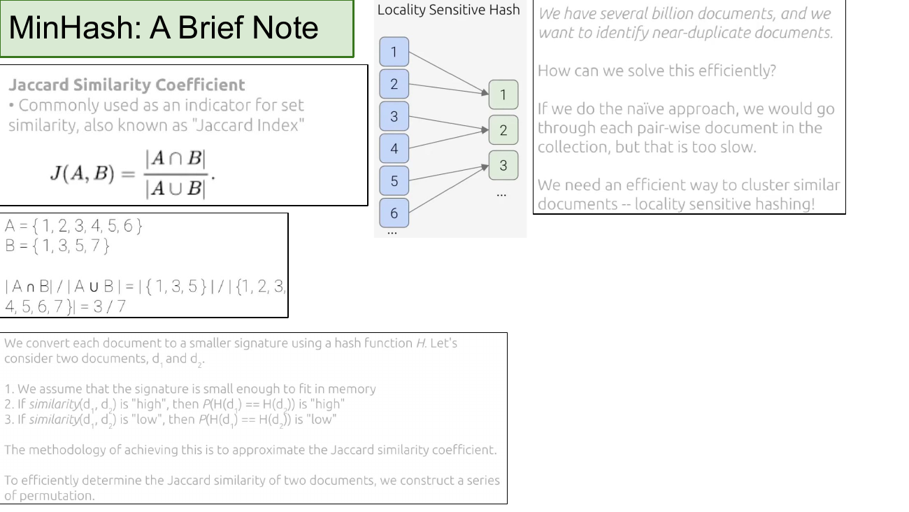
On the slide

A brief primer on the deduplication trick every one of these pipelines uses. Jaccard similarity measures set overlap: $J (A, B) = \frac{| A \cap B |}{| A \cup B |}$ . MinHash + Locality-Sensitive Hashing gives you an approximation of this in sublinear time by bucketing "similar" documents into the same hash.

Why you need this at web scale

Naïve near-duplicate detection is O(n²) in the number of documents. For billions of documents that's astronomical. LSH turns it into a constant-time bucket lookup: each doc gets a compact signature, docs with similar signatures land in the same bucket, and you only compare within buckets. The math trick is that MinHash signatures preserve Jaccard similarity in expectation, so hash collisions correlate with real overlap.

→ Related

Broder's 1997 paper On the Resemblance and Containment of Documents is the original; practically every modern dedup pipeline traces back to it. Cited in the seminar's bibliography.

§4From curation to synthesis: the pivot.

Slides 12–15 are the transition. Curation has diminishing returns — you can only wring so much more quality out of the same finite web. Once you accept that, the next move is getting a model to write the training data. That split runs along the two big LLM training stages (pretraining vs post-training) which get a terminology-clarification slide, plus a brief note on The Pile as pretraining-era context.

Slide 12 / 34

From Curation to Synthesis. Text: we've seen pure curation attempts and why curation is necessary; now we pivot to actual generation and synthesis of data. Until now we spoke about deciding what data trains the models; now we move to a model itself writing the data that trains models. Generation splits into two stages: pretraining and post-training. Two plots from FineWeb: HellaSwag Acc vs Training tokens (billions) for various filter strategies showing diminishing returns; Aggregate Acc vs Training tokens for RefinedWeb, Global minhash, Base filtering. Yellow note: visuals from FineWeb illustrating diminishing returns of more training tokens on the same model.

slide 12 · why you eventually run out of curation runway

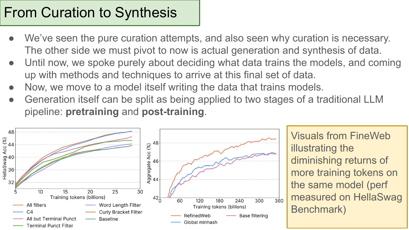
On the slide

The two FineWeb plots show the same story from different angles: as you add training tokens, benchmark accuracy climbs but the slope flattens. Doubling your tokens no longer doubles your quality. And you can only add tokens up to a point — the web is finite.

What to take from it

This is the empirical case for pivoting to synthesis. If curation gives you diminishing returns and the upstream pool is bounded, the next lever is generating new tokens. The split Vishal draws — one synthesis paper for pretraining (WRAP), two for post-training (Self-Instruct, Evol-Instruct) — mirrors the two stages of modern LLM training, and each stage needs a different kind of synthetic data.

Slide 13 / 34

Section divider slide: Generation — Because my supplier cut me off :(

slide 13 · section divider — Generation

On the slide

Section header for the synthesis block, with a joke subtitle about the web running dry. Curation being exhausted is exactly the "supplier cut me off" scenario.

What to take from it

You reach for synthesis for one of three reasons: (a) the domain is under-represented on the public web, (b) the format you need isn't naturally in the web (e.g. instruction-following pairs), or (c) you're out of tokens. WRAP is a (c) paper, Self-Instruct is a (b) paper, and most industry work is quietly all three at once.

Slide 14 / 34

Terminology Clarifications. Pre-training: singular task of next-token prediction, self-supervised; product is a model that continues text but can't follow instructions or hold a conversation. Post-training: second phase where a raw pre-trained base is refined using curated datasets and feedback to safely follow instructions, hold conversations, and perform specific tasks; supervised. Average zero-shot accuracy: run a suite of downstream tasks with no in-context examples, score, average across tasks; tests pretraining, not in-context learning. Perplexity: exponential of average negative log-likelihood per token; informally, how many equally likely options the model was choosing between at each step; a perplexity of 10 means it was about as uncertain as picking uniformly among 10 tokens. C4 Dataset: heuristic filterings of a 2019 crawl — drop lines without terminal punctuation, that mention javascript, or have terms of use / cookie policy statements; drop docs that were too short or contained lorem ipsum or a curly bracket.

slide 14 · terminology clarifications

On the slide

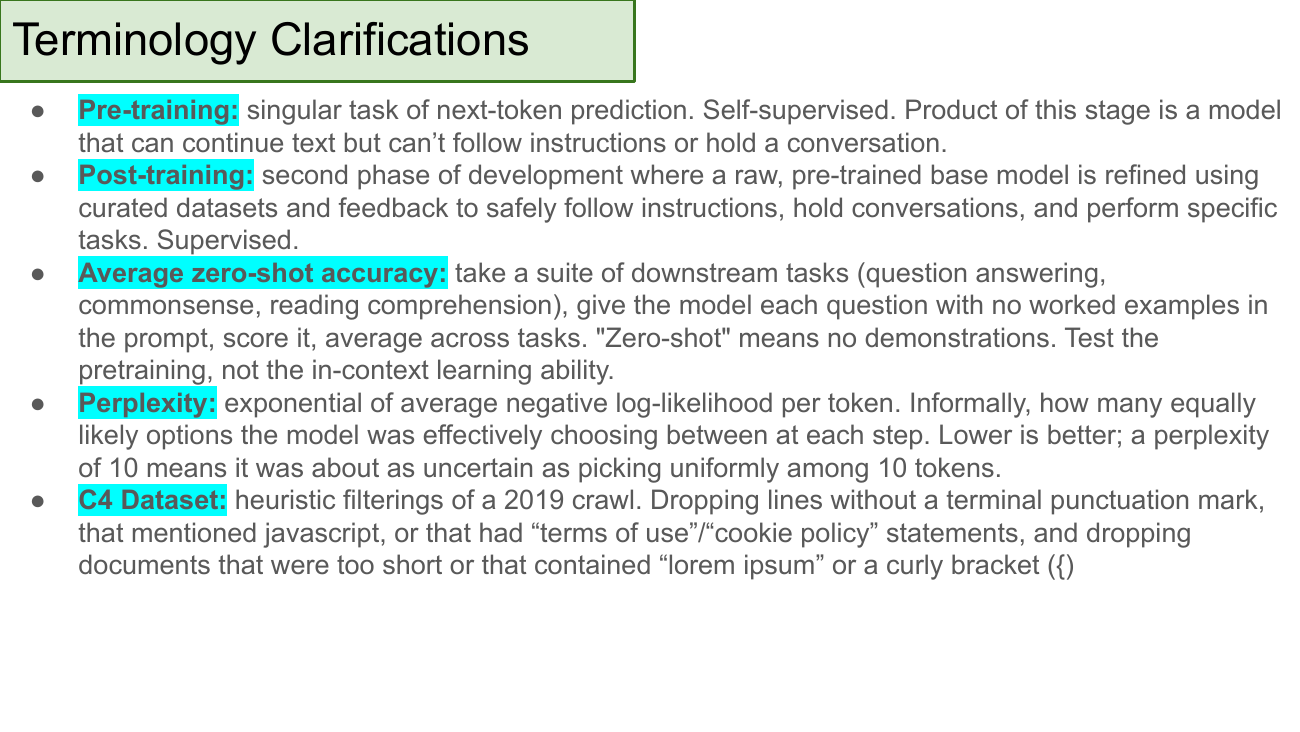
Five terms that will appear on every subsequent slide. Pre-training is the self-supervised next-token pass that produces a base model. Post-training is the supervised refinement (SFT, RLHF, DPO) that produces a chat-shaped model. Zero-shot accuracy measures the pretraining, not the in-context learning ability. Perplexity is the standard pretraining metric — lower is better, and PPL=10 means the model was about as uncertain as picking uniformly among 10 tokens. C4 is the heuristic-filtered 2019 crawl that a lot of prior work uses as its baseline dataset.

Why this slide is worth reading

Every subsequent chart splits performance by "pretraining" vs "post-training" and reports numbers in either perplexity or zero-shot accuracy. Getting these five terms nailed down here saves a lot of re-reading later.

⚠ Watch out

"Zero-shot" in this context means no worked examples in the prompt, not "we tested on data the model never saw". That second meaning gets its own section (§8 · Decontamination). Two different senses, same word.

Slide 15 / 34

The Pile: A Brief Note. 825.18 GiB English text dataset composed of 22 diverse, high-quality subsets — established NLP datasets plus several new ones — for training and as a broad-coverage benchmark. A treemap shows Composition by Category with big blocks for PubMed Central, ArXiv, Pile-CC, OpenWebText2, StackExchange, Wikipedia, DM Math, Github, and smaller blocks for Bibliotik, PG-19, BC2, Subtitles, HN, YT, IRC, EP, FreeLaw, USPTO, PMA, Phil, NIH. Bullets note it's curated to teach LLMs foundational language and cross-domain knowledge during pretraining; introduced here because it forms the perplexity test set in the WRAP paper covered next. Reference: The Pile: An 800GB Dataset of Diverse Text for Language Modeling.

slide 15 · The Pile as context for WRAP

On the slide

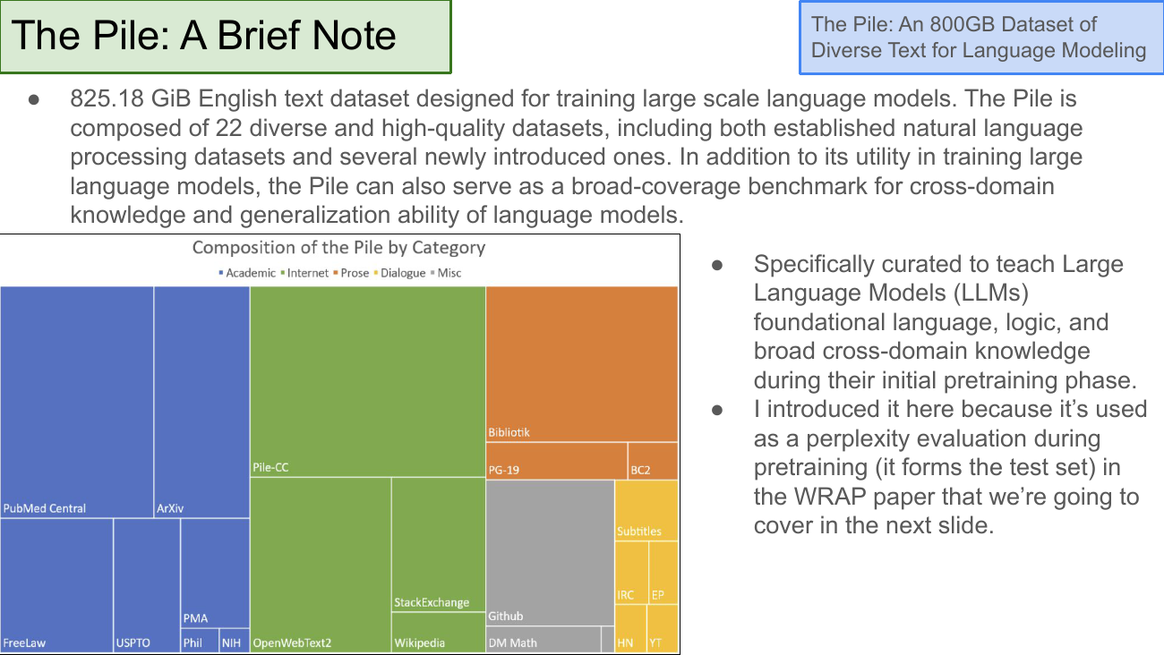
The Pile is an 800 GB, 22-subset English corpus assembled by EleutherAI in 2020. The treemap shows what's in it: heavy on academic text (PubMed, ArXiv), reasonable amounts of code (GitHub) and general web (Pile-CC), and smaller specialist slices (Enron emails, HackerNews, YouTube subtitles).

Why it's on the deck

The Pile is what the WRAP paper (next slide) uses as its perplexity test set. The 22-subset construction is also historically interesting as an early "mixture-of-domains" pretraining set — a precursor to modern data mixtures like DCLM-Baseline + StarCoder + ProofPile2 you saw on slide 9.

§5Synthesis for pretraining: WRAP — rewrite the web.

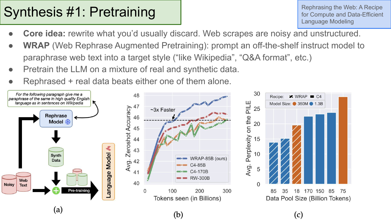
The first synthesis paper is WRAP (Web Rephrase Augmented Pretraining). Its argument is minimalist: the web is noisy, so take a strong instruct model, ask it to rephrase web text into a target style (Wikipedia-like, Q&A format), and train on a mixture of real and rephrased. The claim is that the mixture beats either alone.

Slide 16 / 34

Synthesis #1: Pretraining (WRAP). Core idea: rewrite what you'd usually discard — web scrapes are noisy and unstructured. WRAP (Web Rephrase Augmented Pretraining): prompt an off-the-shelf instruct model to paraphrase web text into a target style (like Wikipedia, Q&A format). Pretrain the LLM on a mixture of real and synthetic data. Rephrased + real beats either one alone. Three panels: (a) a pipeline showing noisy web text going through a rephrase model with a prompt to convert to Wikipedia-style, producing synth data that mixes with real for pretraining; (b) a plot Avg Zeroshot Accuracy vs Tokens seen, WRAP-85B reaches ~46 acc ~3x faster than C4-85B / C4-170B / RW-300B; (c) a bar chart Avg Perplexity on the PILE vs Data Pool Size, WRAP recipe beats C4 across 85, 35, 18B pools at 350M and 1.3B models. Reference: Rephrasing the Web: A Recipe for Compute and Data-Efficient Language Modeling.

slide 16 · WRAP — rephrase-and-mix

On the slide

WRAP in three panels. (a) The pipeline: noisy web goes through a frozen instruct model (Mistral) that's prompted to paraphrase into "high-quality English like Wikipedia". Output is synth data, mixed with real data, used as the pretraining set. (b) Zero-shot accuracy vs training tokens: WRAP-85B hits the accuracy of C4-170B/RW-300B roughly 3× faster. (c) Perplexity on The Pile: WRAP recipe beats C4 across data-pool sizes.

Why the mixture beats either alone

Real data is diverse but noisy. Synthetic paraphrases are clean and well-formatted but tend to collapse in style (everything ends up sounding like the Wiki prompt). The mixture inherits diversity from the real half and signal density from the synthetic half. Faithfulness comes from the real provenance of the source; diversity comes from not throwing away the original.

✦ Key takeaway

WRAP is the cleanest existing evidence that rewriting web text — not just filtering it — is a lever. And it costs 3× fewer training tokens for the same benchmark score. That's a big win in a world where tokens are becoming the scarce resource.

Slide 17 / 34

Left column: jointly train the LLM on real and synthetic data and investigate the impact of rephrasing on model performance. Rephrased synthetic data has higher utility (fewer tokens suffice) than just real data because it (1) incorporates style diversity that closely reflects downstream evaluation style; (2) has higher signal density — raw web text is padded with boilerplate, typos and malformed structure, a cleaned paraphrase carries the same content in fewer, better-formed tokens. Right column: two perplexity bar charts across Wiki, OWT2, Books2, Books, ArXiv, StackX, Github, Math, HNews, Enron, Pubmed-C, Ubuntu, Pubmed-A, FreeLaw, NIH, USPTO, PG-19, Phil, Youtube, OpenSubs, CC showing consistent improvements from adding C4+QA-85B and C4+Med-35B mixtures.

slide 17 · why the WRAP mixture actually helps

On the slide

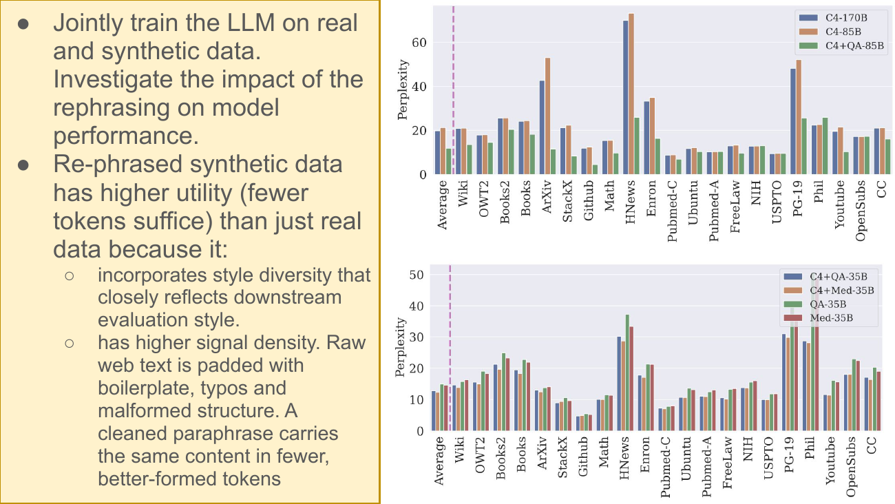
Two more perplexity plots, this time broken down by domain. C4+QA-85B (real + Q&A-style rephrases) beats C4 alone on almost every Pile subset. The pattern holds even when you swap the rephrase style (C4+Med-35B, medical-style rephrasing).

The two reasons rephrased data helps

Style diversity aligned with evaluation. Downstream evals tend to be in Wikipedia or Q&A style. Rephrased data biases the model toward those styles.
Signal density. A well-formed paraphrase says the same thing as a raw web dump but in fewer, cleaner tokens. Fewer tokens per unit of content = the model learns more per gradient step.

⚠ Watch out

This slide has the hidden setup for §7 (model collapse). WRAP works because the rephraser is stronger than the trainee, and because you keep the real data in the mix. Break either assumption — recursively rephrase, or throw away the real data — and the whole thing collapses. That's exactly the failure Shumailov et al. document.

§6Synthesis for post-training: Self-Instruct & Evol-Instruct.

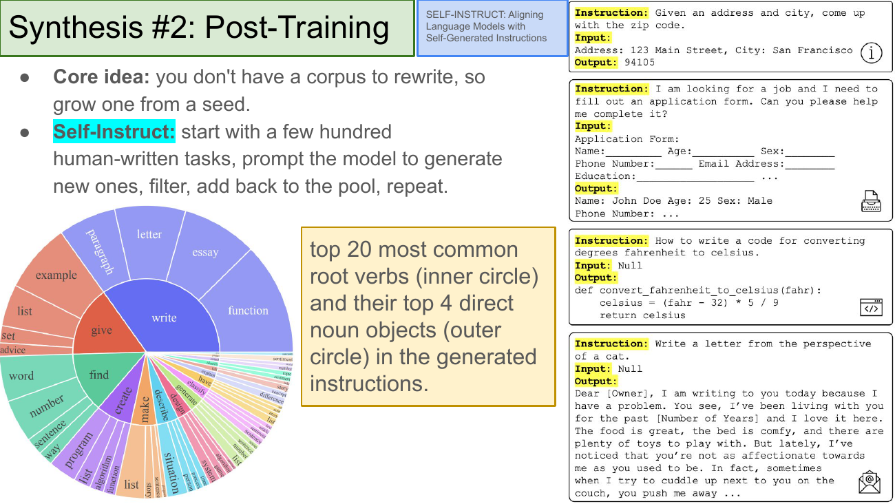
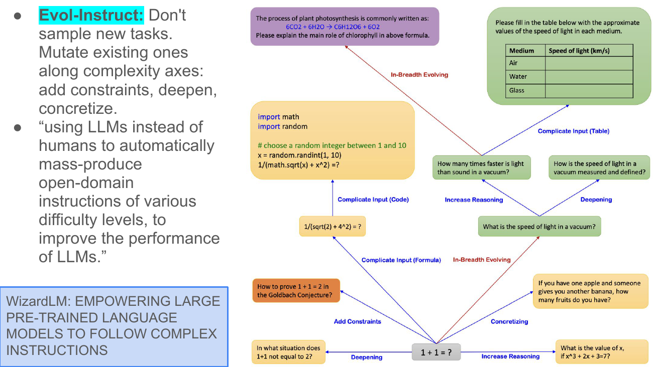
For post-training there's no big web corpus to paraphrase — instruction-response pairs mostly don't exist in the wild. So slides 18–20 cover two techniques that grow a dataset from a seed. Self-Instruct (2022) bootstraps thousands of new tasks from a few hundred human ones. Evol-Instruct / WizardLM (2024) doesn't invent new tasks — it mutates existing ones along complexity axes.

Slide 18 / 34

Synthesis #2: Post-Training. Core idea: you don't have a corpus to rewrite, so grow one from a seed. Self-Instruct: start with a few hundred human-written tasks, prompt the model to generate new ones, filter, add back to the pool, repeat. Bottom-left: a sunburst chart of the top 20 most common root verbs (write, give, find, create, make, describe, classify, generate, design, have) and their top 4 direct noun objects in generated instructions. Right: four example instruction-input-output tuples: zip code lookup, filling a job application form, converting fahrenheit to celsius as code, writing a letter from the perspective of a cat. Reference: SELF-INSTRUCT: Aligning Language Models with Self-Generated Instructions.

slide 18 · Self-Instruct — grow tasks from a seed

On the slide

Self-Instruct in one screen. Sunburst on the left shows the verb-noun diversity of the generated tasks (write letters, give quotes, find zip codes, classify text, generate code). The four boxes on the right are actual instruction-input-output examples the pipeline emitted.

Why bootstrap from a seed

The alternative — hire humans to write 50,000 instruction pairs — is expensive and slow. Self-Instruct uses a strong model to imitate the seed style and produce many more examples for cheap. The trick is that even a small human seed pins down what "an instruction" is supposed to look like; the model then generates variations, and a filter throws out the low-quality ones.

Slide 19 / 34

Self-Instruct pipeline diagram. 175 seed tasks with 1 instruction and 1 instance per task → Task Pool. Step 1: Instruction Generation — LM samples the pool and generates a new task instruction (Example: Give me a quote from a famous person on this topic). Step 2: Classification Task Identification — LM decides whether the new task is a classification task. Step 3: Instance Generation — if Yes go Output-first (generate class label like Pro-abortion then Input like a text about abortion rights); if No go Input-first (generate input like Topic: importance of being honest, then Output like a Thomas Jefferson quote). Step 4: Filtering — filter low-quality or similar generations, add valid ones back to the task pool, repeat. Caption: the resulting data can be used for instruction tuning of the language model itself.

slide 19 · Self-Instruct pipeline in detail

On the slide

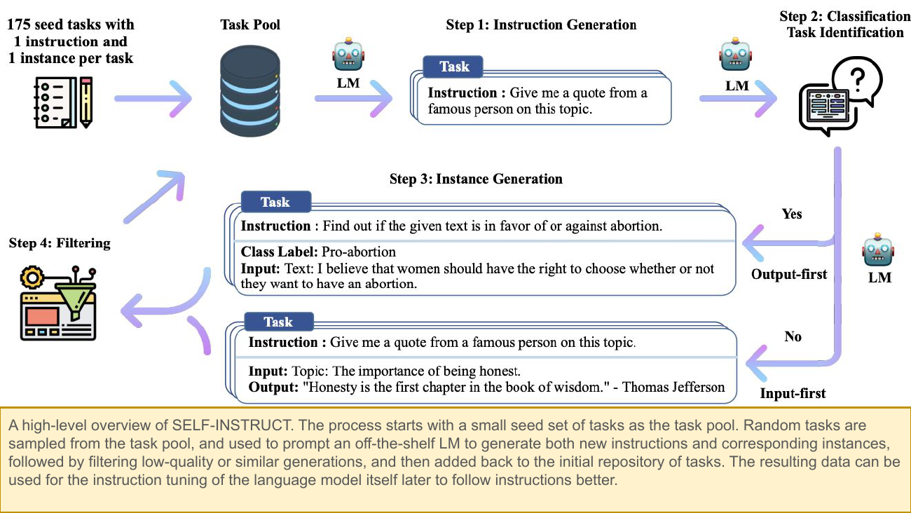
The four steps drawn as a loop. 175 human seeds → Instruction Generation (LM writes a new instruction) → Classification Task Identification (is this a labelling task?) → Instance Generation (Output-first if classification, Input-first otherwise) → Filtering (drop near-duplicates and junk) → back into the pool.

Why the classification split matters

For classification tasks, generating a random input and then labelling it makes the labels imbalanced — you'd get 90% "positive" reviews because the model tends to write positive-sounding text. Instead, Self-Instruct generates the label first and then constructs an input that fits it. This is a small but important trick: it's how the pipeline preserves label diversity, which is a specific facet of the general diversity requirement.

Under the hood

The filter step is what keeps this from being pure amplification of the model's biases. Every new generation is checked against the existing pool for near-duplicate instructions (ROUGE overlap) and for basic quality signals (well-formed, non-empty output, executable code where relevant). Failures go in the bin; passes go in the pool. Iterate.

Slide 20 / 34

Evol-Instruct: don't sample new tasks, mutate existing ones along complexity axes — add constraints, deepen, concretize. Quote: using LLMs instead of humans to automatically mass-produce open-domain instructions of various difficulty levels to improve LLM performance. Right: a tree diagram showing 1+1=? being evolved via Deepening, Add Constraints, Increase Reasoning, Concretizing, In-Breadth Evolving, Complicate Input (Formula/Code/Table). Examples: 'In what situation does 1+1 not equal 2?', 'How to prove 1+1=2 in the Goldbach Conjecture?', 'If you have one apple and someone gives you another banana, how many fruits do you have?', '1/(sqrt(2)+4^2) = ?', 'What is the value of x, if x^3 + 2x + 3 = 7?', 'How many times faster is light than sound in a vacuum?', 'Please fill in the table below with the approximate values of the speed of light in each medium'. Reference: WizardLM: Empowering Large Pre-Trained Language Models to Follow Complex Instructions.

slide 20 · Evol-Instruct — mutate existing tasks harder

On the slide

Evol-Instruct starts from a simple seed instruction and applies one of several evolution operators: add constraints, deepen, concretize, increase reasoning, complicate input (with a table, code snippet, or formula), or in-breadth evolve (jump to a new domain). The 1+1=? tree shows the same seed producing seven wildly different, harder tasks.

Why mutate instead of sample

Self-Instruct pushes for breadth — new task types. But it doesn't obviously get you hard tasks; the generator's easiest outputs dominate. Evol-Instruct pushes for depth along a controlled axis. The claim of WizardLM is that a model trained on the evolved instructions inherits the harder capability. In practice most modern post-training datasets are a mix of the two styles.

→ Related

Wang et al., Self-Instruct (ACL 2023, arXiv:2212.10560) and Xu et al., WizardLM (ICLR 2024, arXiv:2304.12244). Both are in the bibliography.

§7Student, teacher, and model collapse: the failure mode.

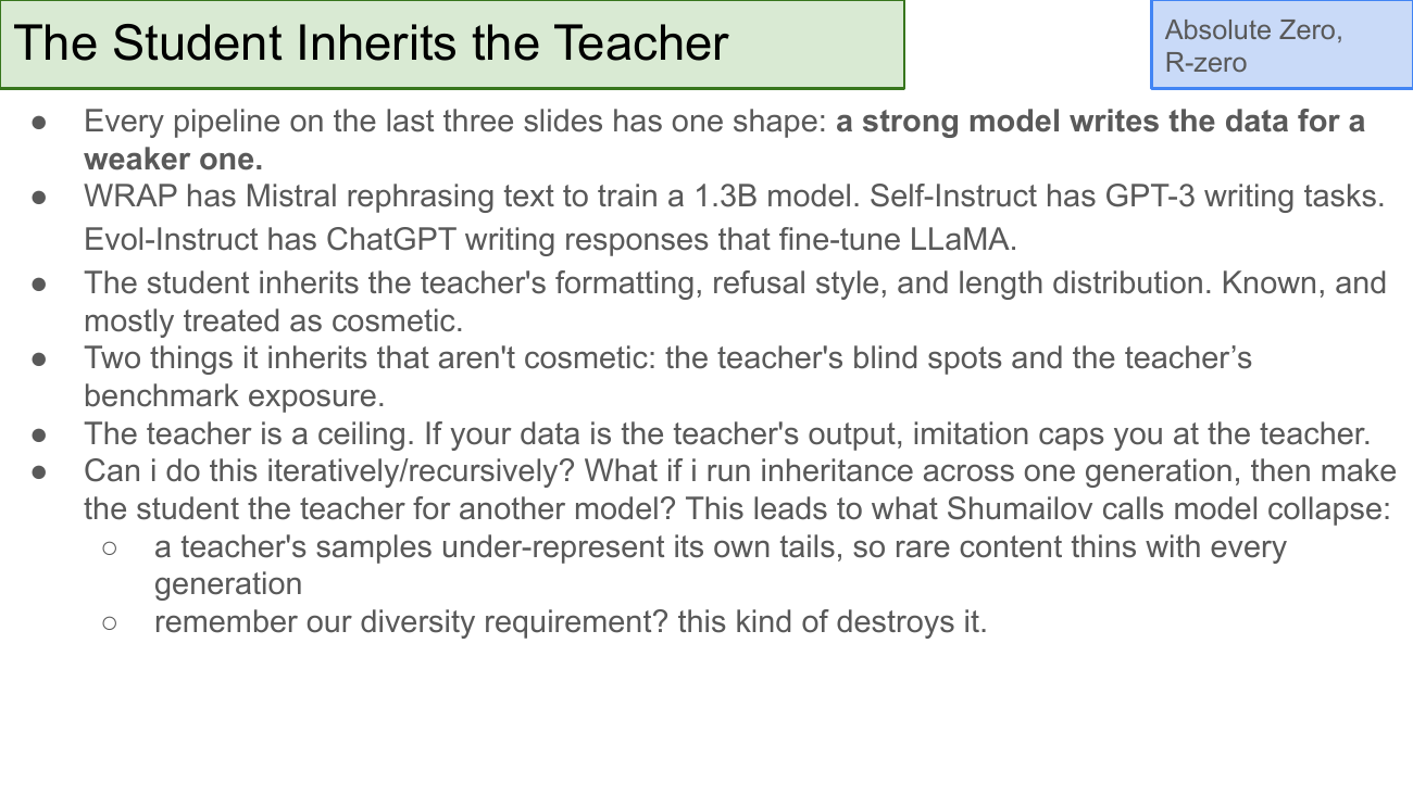
Slides 21–25 name the failure mode that all three synthesis techniques quietly risk. Every pipeline so far has the same shape: a strong teacher writes the data for a weaker student. What if you iterate — the student becomes the teacher for the next generation? Shumailov et al. (Nature 2024) show the tails of the data distribution shrink each generation until the model collapses onto a narrow high-probability mode. Gerstgrasser et al. (COLM 2024) show one clean fix: don't replace, accumulate.

Slide 21 / 34

The Student Inherits the Teacher. Bullets: every pipeline in the last three slides has one shape — a strong model writes data for a weaker one. WRAP has Mistral rephrasing text to train a 1.3B model. Self-Instruct has GPT-3 writing tasks. Evol-Instruct has ChatGPT writing responses that fine-tune LLaMA. The student inherits the teacher's formatting, refusal style, length distribution — mostly cosmetic. Two things it inherits that aren't cosmetic: the teacher's blind spots and the teacher's benchmark exposure. The teacher is a ceiling — imitation caps you at the teacher. Can I do this iteratively/recursively? Run inheritance across one generation, then make the student the teacher for another model — this leads to what Shumailov calls model collapse: teacher's samples under-represent its own tails, so rare content thins with every generation; destroys the diversity requirement. Reference: Absolute Zero, R-zero.

slide 21 · the strong-writes-for-weak pattern

On the slide

Vishal steps back and names the pattern: WRAP, Self-Instruct, Evol-Instruct all have a strong model writing the data for a weaker one. Cosmetic inheritance (formatting, refusal style, length distribution) is fine. Non-cosmetic inheritance — the teacher's blind spots and its benchmark exposure — is not.

Why the recursive case breaks

A single generation is fine because you have a real ceiling (the teacher) and real ground (the human seed). Do it iteratively — student becomes next generation's teacher — and both the ceiling and the ground drift. Rare events get under-represented at every step, and the model progressively "forgets" the tails of the distribution. Diversity, our second quality axis, dies.

✦ Key takeaway

Imitation caps you at the teacher — you can't exceed the model you're copying from. That alone justifies fresh human data even in a synthesis-heavy pipeline. Recursion makes it worse: not only can you not exceed the teacher, you actively degrade with every generation.

Slide 22 / 34

Model Collapse: The Failure. Training recursively on model-generated content causes irreversible defects in the resulting models, in which tails of the original content distribution disappear. Left: a chain diagram showing Data^0 (real) → Model 0 → Data^1 (model-generated) → Model 1 → ... → Data^n → Model n; over time Data^0 ≈ Data^1 ≈ ... ≈ Data^n. Right: a failure loop — probable events are overestimated, improbable events are underestimated; finite sampling → approximate fitting → data^n → model^n; probable events poison reality, tails shrink over time. Three yellow boxes explain the three error sources: Statistical approximation error (non-zero probability of losing rare events at every resampling step), Functional expressivity error (model class can't represent true distribution), Functional approximation error (optimizer / SGD doesn't land on truth).

slide 22 · Shumailov's diagnosis of model collapse

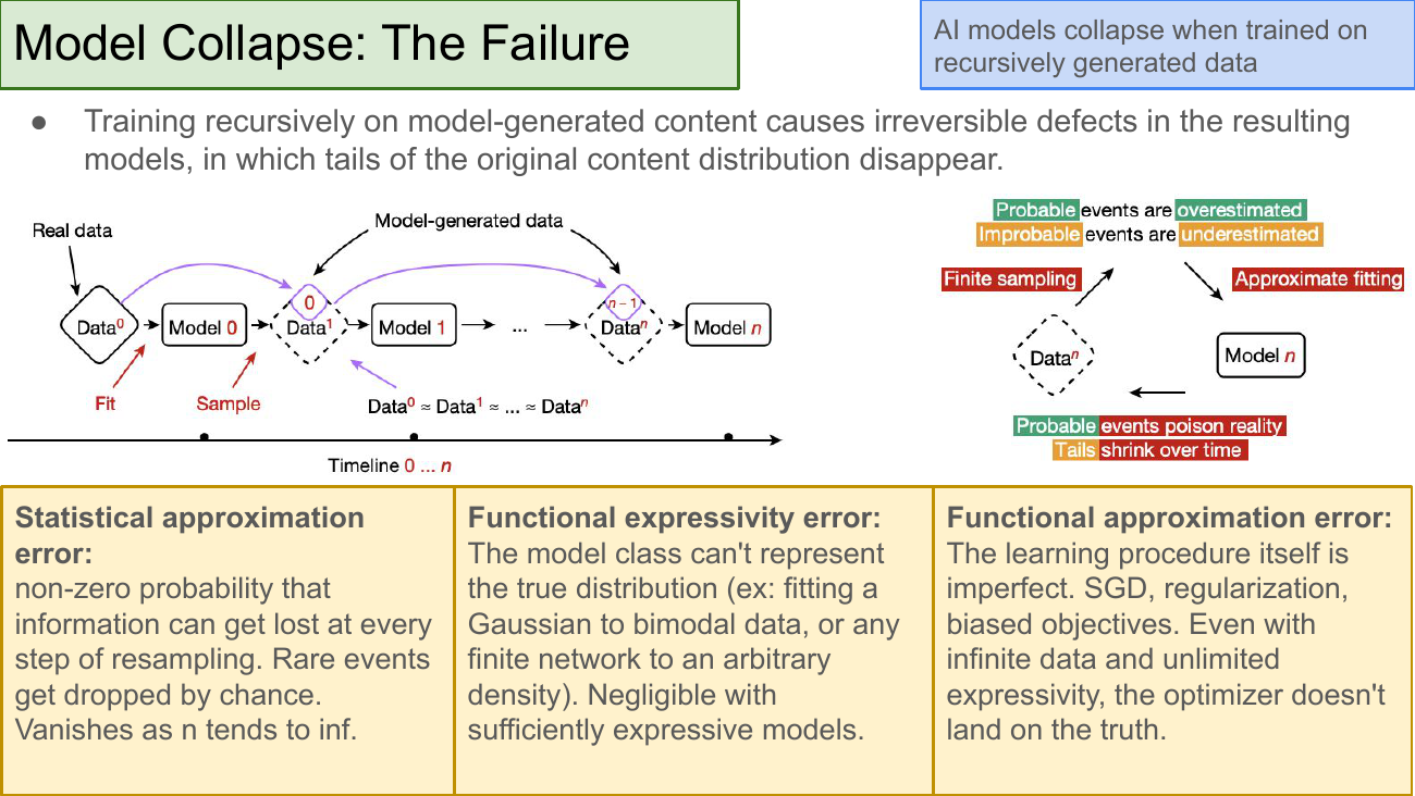
On the slide

The mechanism, drawn as a chain. At each generation $n$ , you fit a model to ${Data}^{n}$ , sample new data from it, and use that to fit the next generation. The right-side loop shows why the process is self-poisoning: probable events get over-sampled, improbable ones get dropped, and the process compounds. Three error sources drive it: statistical (finite-sample noise), functional expressivity (model class can't fit the true distribution), functional approximation (optimiser doesn't converge to the truth).

Why "irreversible" is doing work in the abstract

The paper's word is irreversible. Once the tails have been sampled out, no amount of further training on the collapsed distribution can bring them back. The information about rare events is genuinely gone from the training set. You can only recover by injecting fresh real data — which is exactly the Gerstgrasser fix on slide 24.

→ Reference

Shumailov, Shumaylov, Zhao, Papernot, Anderson & Gal, AI Models Collapse When Trained on Recursively Generated Data, Nature 631:755–759, 2024.

Slide 23 / 34

Two perplexity histograms from Shumailov et al. Left panel (b): No data preserved, five epochs. Perplexity of generated data points evaluated by a model trained with real wikitext2, colored by generations 0, 1, 2, 3, 5, 9. As generations progress, mass shifts leftward (toward low perplexity) and the tail shrinks; tall narrow spikes appear at very low perplexity, indicating a handful of sequences dominating. Right panel (c): 10% data preserved, ten epochs. Same experiment but keeping 10% real data each generation — the leftward drift still happens but much weaker, the hump keeps its shape and the tail survives. Note: consistent with WRAP; the mixture is better than the parts.

slide 23 · collapse in a picture (and the first hint of the fix)

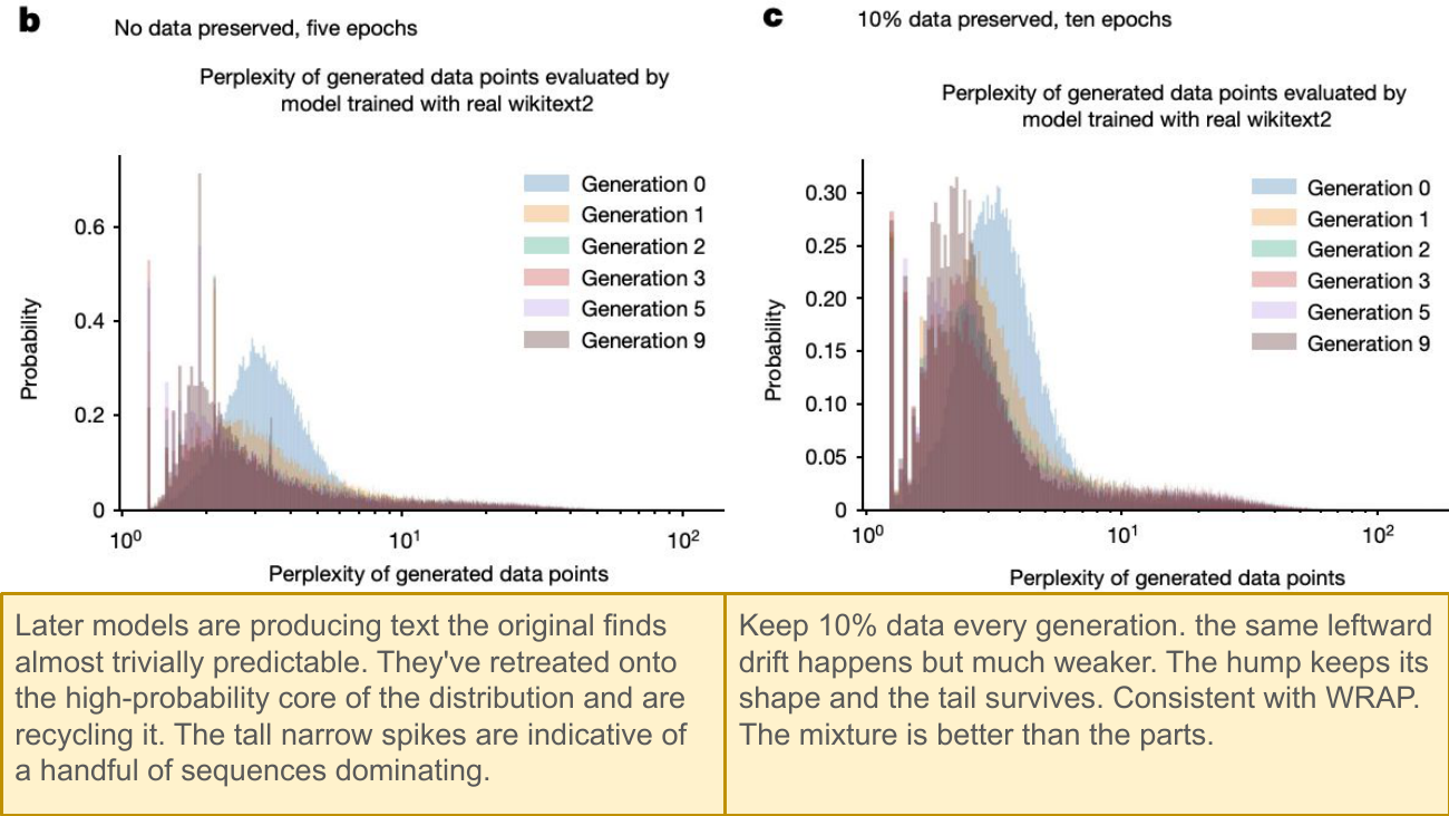
On the slide

Two perplexity histograms. Panel (b) shows what happens when you replace all training data each generation: the distribution shifts left (the model finds everything trivially predictable) and grows tall, narrow spikes (a few sequences dominating). Panel (c) shows the same experiment but keeping 10% real data every generation: the shape mostly survives, the tail is preserved.

What to take from it

The two panels together are the empirical case for both the disease and the cure. Pure recursive synthesis collapses; mixing in a real-data fraction each generation stops the collapse. That's the WRAP finding again in a different setting, and it sets up the Gerstgrasser paper on the next slide.

Slide 24 / 34

Can We Avoid Model Collapse? Text: instead of new data replacing old data, what if we accumulated instead? Empirically, accumulating successive generations of synthetic data alongside the original real data avoids model collapse — consistent with the right-side figure on the previous slide. Two plots side by side of Cross Entropy (Test) vs Model-Fitting Iteration (1-5) for Language Models Pretrained on TinyStories, comparing four model sizes GPT-2 9M, Llama-2 12M/42M/126M. Left (Replace): test loss steadily rises across iterations for all sizes. Right (Accumulate): test loss stays flat or drifts slightly downward. Reference: Is Model Collapse Inevitable? Breaking the Curse of Recursion by Accumulating Real and Synthetic Data.

slide 24 · Gerstgrasser's accumulate-don't-replace fix

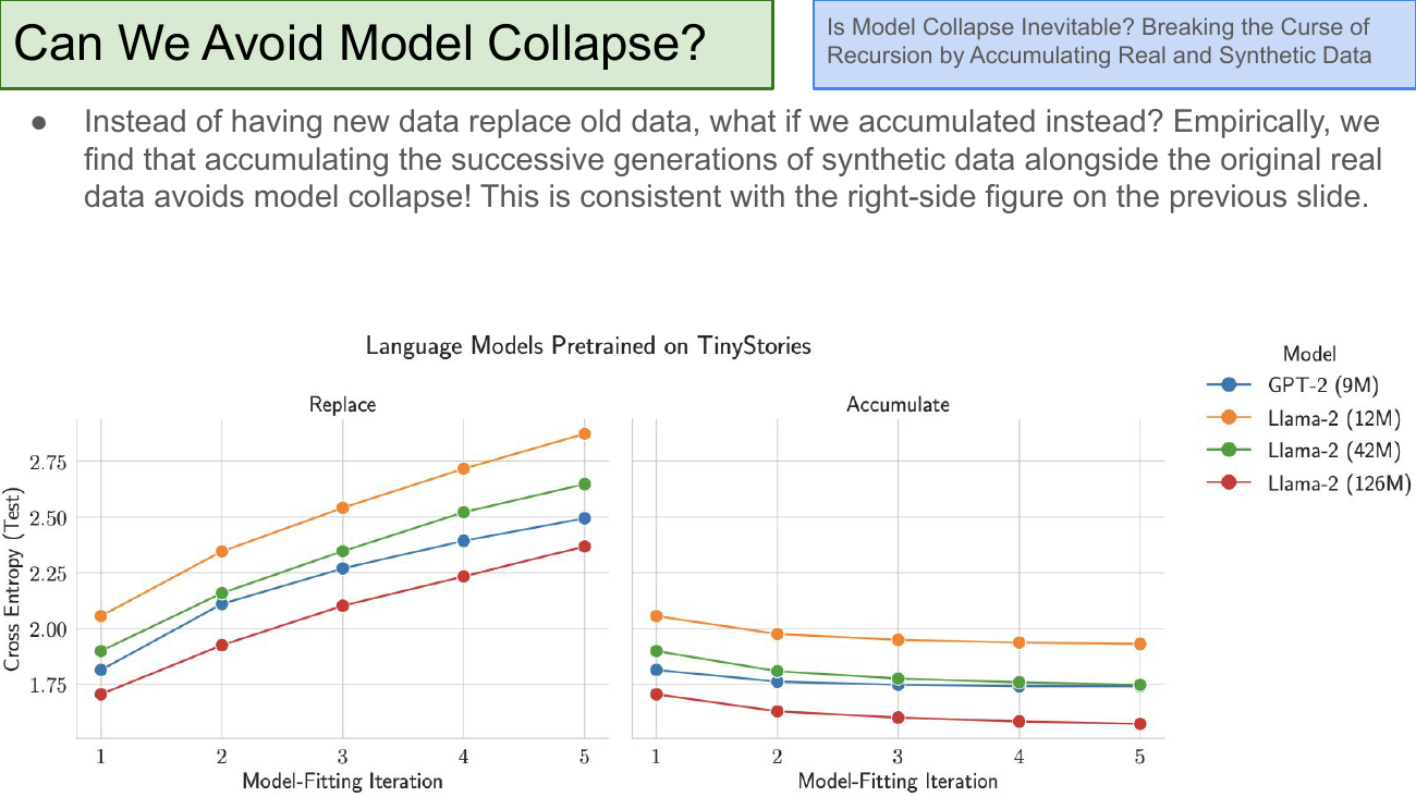
On the slide

Gerstgrasser et al. run the recursion experiment twice — once replacing data each generation, once accumulating. Replace: test loss climbs monotonically across generations for every model size. Accumulate: test loss stays roughly flat or even drifts down.

Why accumulation fixes what replacement breaks

The Shumailov chain has each generation depend only on the previous one's outputs. Any information that gets sampled out is gone forever. When you accumulate — keep all previous generations of data including generation zero (real data) — the real distribution stays in the mix. The model trains on a superset that always contains the ground truth. Tails don't shrink because they're structurally preserved in the historical data.

✦ Key takeaway

The choice of "replace vs accumulate" is basically the difference between "collapse guaranteed" and "collapse avoided". Both papers converge on the same prescription: keep real data in the training set at every generation.

Slide 25 / 34

Two column diagram from Gerstgrasser paper: Replace Data (left) and Accumulate Data (right). Replace: Model 1 fit to Data 1 (real), then samples Data 2 (model-generated) which trains Model 2, which samples Data 3, etc. Only the latest generation's data is used. Test Loss vs Model-Fitting Iteration curves rising. Accumulate: same chain, but at each iteration the training set is the union of Data 1 (real) plus all previous synthetic generations. Test Loss curve is flat across iterations. Legend on the right explains the color coding: pink Model, green Training Data, yellow Real Data, blue Model-Generated Data; solid arrows for Fit, dashed arrows for Sample.

slide 25 · the same story as a single figure

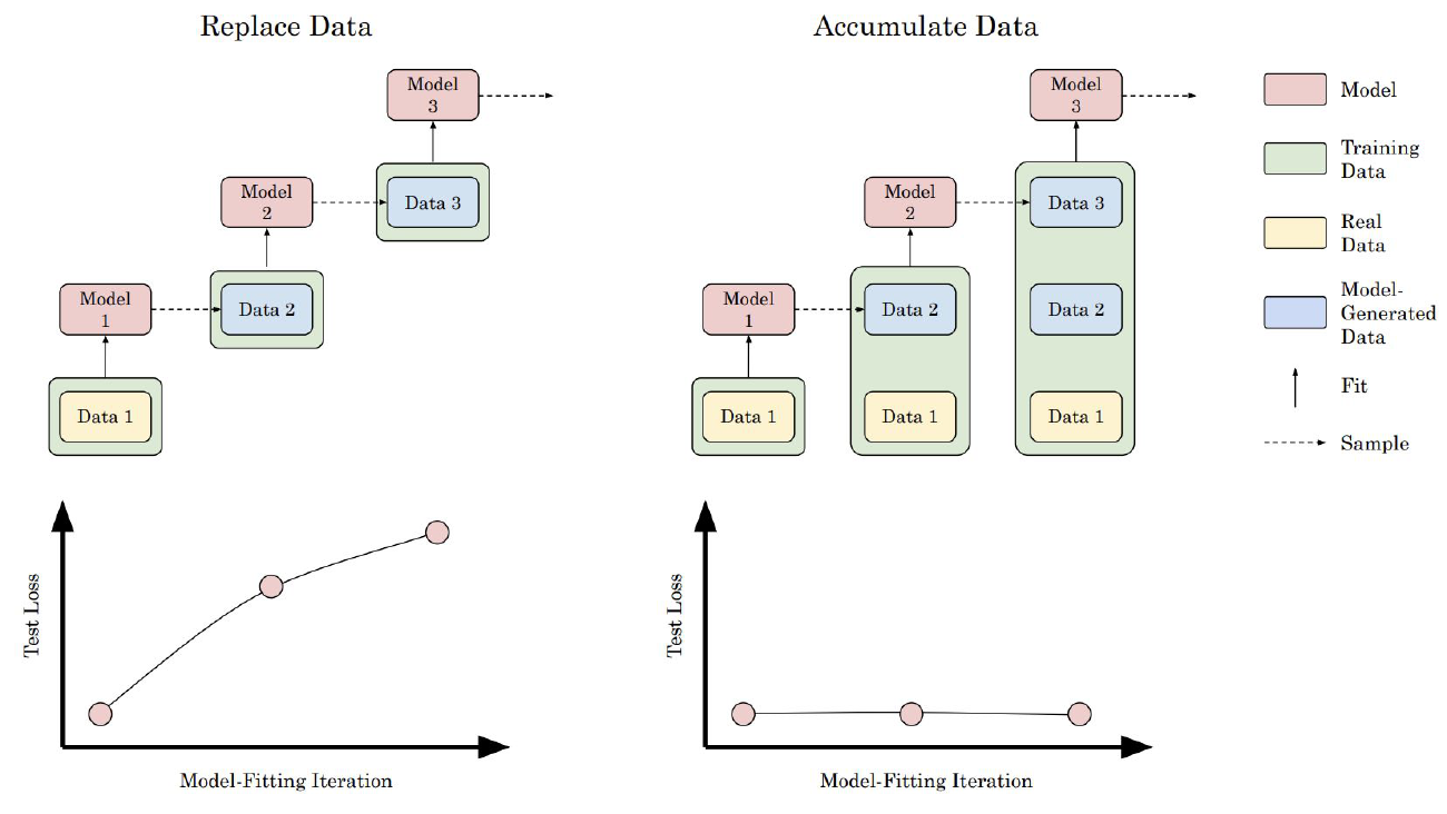
On the slide

The Gerstgrasser figure that summarises both slides. On the left, the "replace" chain: each model trains only on its predecessor's samples. On the right, the "accumulate" chain: each model trains on the union of the original real data and all prior synthetic generations. Test loss climbs in the first case, stays flat in the second.

What to take from it

This is the one slide to remember out of the model-collapse section. If your pipeline is designed around "accumulate", collapse basically stops being a threat. If it's designed around "replace", every iteration is a bet against the tails. Modern industrial pipelines all follow the accumulate pattern for exactly this reason.

§8Evaluation & decontamination: the honest hard part.

Every previous section ended with "we know it worked because the benchmark score went up". Slides 26–32 ask the awkward follow-up: can we trust the benchmark? The concern is contamination — training data that includes items from the test set, either literally or as paraphrases. String-matching n-gram filters (what most labs do) miss the paraphrased case completely. An LLM-based decontaminator is proposed as the fix.

Slide 26 / 34

Section divider slide: Evaluation — Personally, I never evaluate because evaluation is a sign of a lack of confidence in your generation and curation.

slide 26 · section divider — Evaluation (with a joke)

On the slide

Section header for the evaluation block. The joke is that evaluation is optional — until it isn't. In practice the field has been running on benchmark-driven ablations for years, and this section is about whether that game is trustworthy.

What to take from it

The pattern established across DCLM, FineWeb, WRAP, and the collapse papers is: change one thing, train a model, score a benchmark, see if the score moved. That protocol only works if the benchmark hasn't leaked into the training set. Which brings us to the next slides.

Slide 27 / 34

Again, how do we know any of this worked? A pattern emerges: DCLM, FineWeb, WRAP, Self-Instruct, model collapse — you train a model, you score a benchmark, over and over. This is the ablation logic the entire field runs on: make a change, see the benchmark score move. We arrive again at benchmark decontamination — the one stage that's technically part of the curation pipeline that no one is incentivized to do correctly. Models score better on datasets released before their training data was collected than on ones released after. Could be a capability gap; could be a leakage warning. Can we trust public benchmarks? Can we trust reported model scores? Are our current methods of evaluation sufficient? How do we decontaminate?

slide 27 · the field's incentive problem

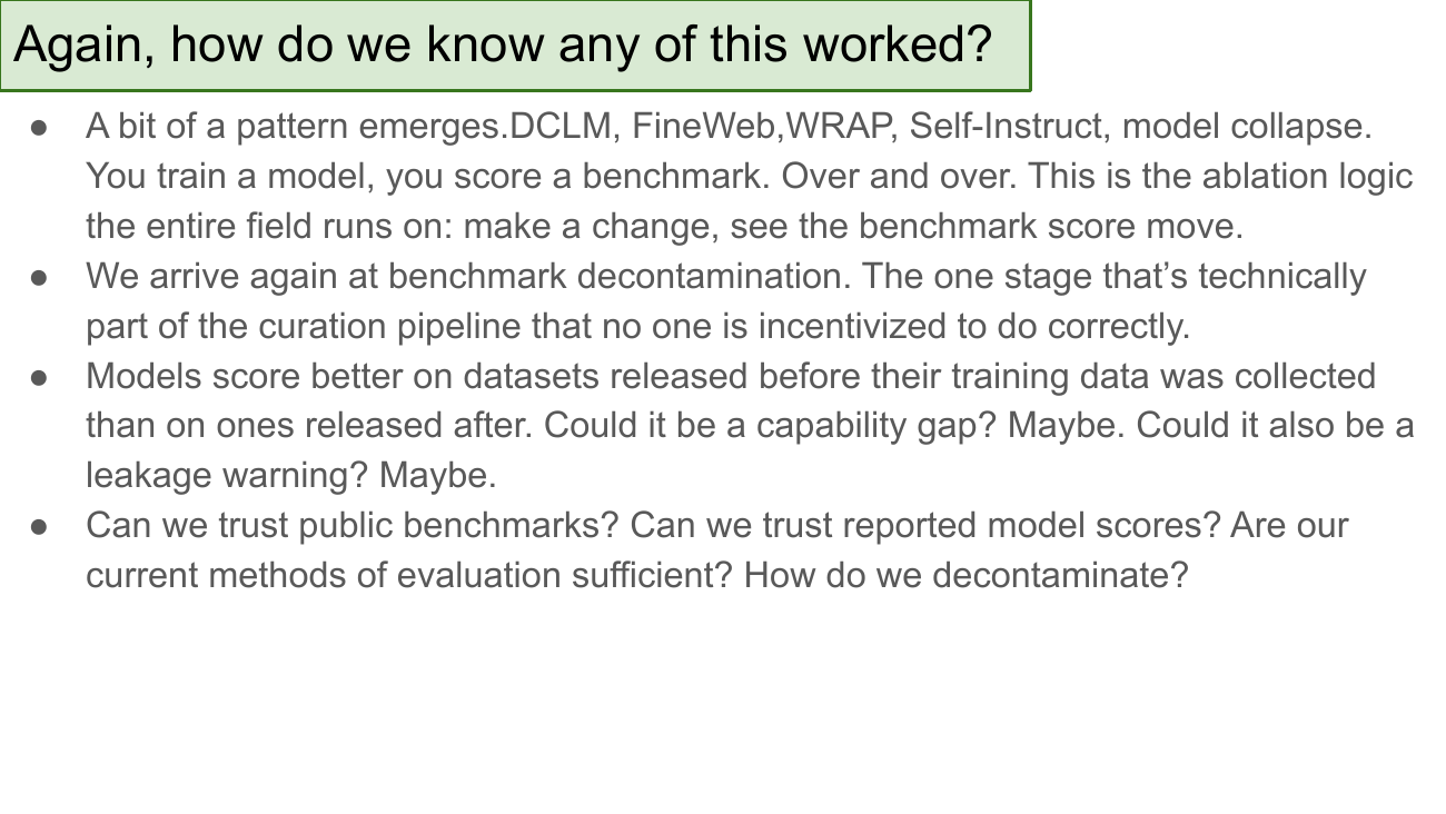
On the slide

Four uncomfortable observations. Ablations depend on benchmarks. Benchmarks depend on decontamination. Nobody is incentivised to decontaminate correctly (better contamination = better numbers). And models consistently score higher on benchmarks released before their training cutoff than on ones released after — which could be a fair capability gap, but could also be a leakage signal.

Why this matters right now

The "benchmarks might be contaminated" concern used to be a niche worry. In 2024 it became a public scandal: several small models posted GPT-4-level scores on MMLU that later turned out to be trained on rephrased test items. The rest of this section is the technical detail of how that happens and what to do about it.

Slide 28 / 34

Benchmark Decontamination. Concerns raised about trustworthiness of public benchmarks due to potential contamination in pre-training or fine-tuning datasets. Most decontamination efforts: string matching (n-gram overlap). Simple variations of test data (paraphrasing, translation) can easily bypass this. Embedding similarity was attempted too: hard to find a good sim threshold. Left panels: MMLU Test Set example, Q: 'Which of the following was a popular reform movement of the 1840s?' with options and answer D, rephrased sample with the same content but different wording answered by 'The movement for abstaining from alcohol' (answer D). Right: a bar chart labeled MMLU showing Llama-2-13B at about 55, Llama-2-13B-rephrase near GPT-4's line at 85. Yellow note: A 13B model can easily overfit a test benchmark and achieve drastically high performance, on par with GPT-4. Ref: Rethinking Benchmark and Contamination for Language Models with Rephrased Samples.

slide 28 · why n-gram overlap misses the real leaks

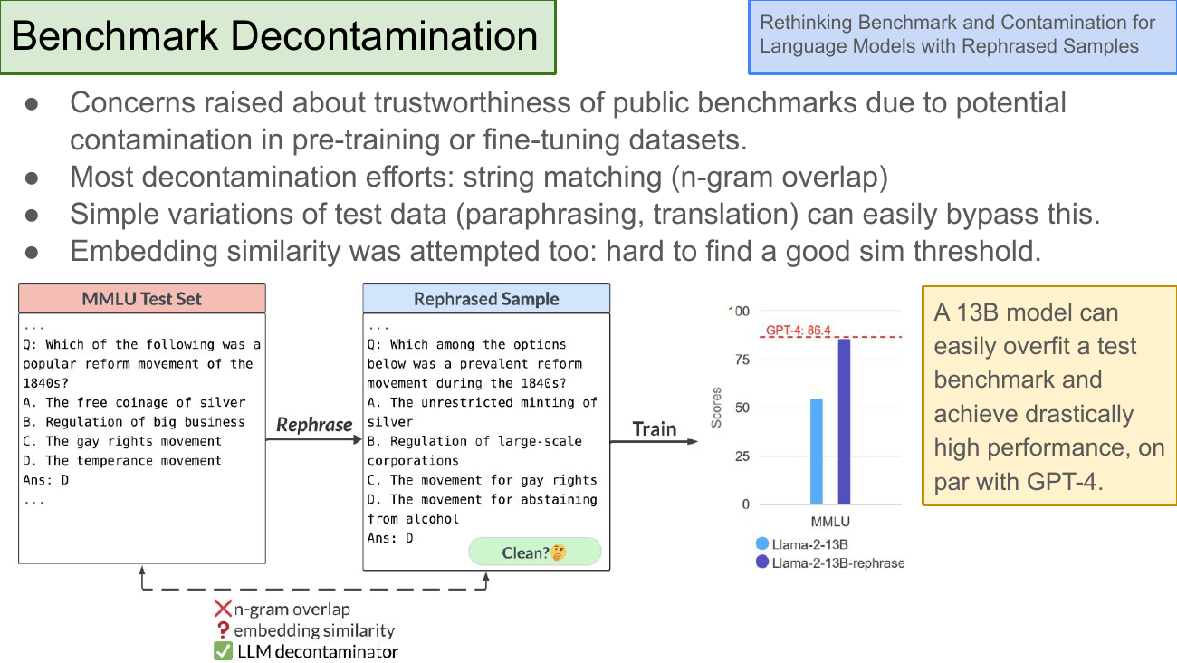
On the slide

The demonstration paper. Standard decontamination uses n-gram overlap between training text and test items. Take an MMLU question, paraphrase it (same semantics, different words), and n-gram overlap drops to zero — decontamination passes. Fine-tune a 13B model on the paraphrases, and it now scores at GPT-4 level on that benchmark. The MMLU score isn't measuring capability at all; it's measuring exposure.

Why this is worse than it looks

Embedding-similarity decontamination catches some paraphrases but throws up too many false positives at useful thresholds. So the field's two default tools both fail: n-gram misses paraphrases, embedding-similarity is too coarse. That means the reported benchmark score of any model whose training set wasn't audited by hand is potentially inflated.

⚠ Watch out

The rephrasing doesn't even have to be adversarial. Any pipeline that uses WRAP-style rephrasing on a web corpus that happens to include benchmark items will accidentally launder them past n-gram filters. Contamination is a bug you can catch by accident.

Slide 29 / 34

Top left: contamination percentages of HumanEval in each training dataset — The Stack (4G subset) 18.9%, StarCoder-Data 15.9%, CodeAlpaca 12.8%, RedPajama-Data (16G) 8.53%. Bottom left: EXAMPLE 1 (GSM-8K Rephrased Sample) showing an original test case about Janet's ducks laying 16 eggs and its rephrased version about Janet's ducks producing 16 eggs each day. Right: yellow note — the paper seeks to investigate whether simple variations of test sets included in the training set could affect benchmark performance. Bar chart of Scores across MMLU, GSM-8k, HumanEval for Llama-2-13B, Llama-2-13B-rephrase, CodeLlama-13B, CodeLlama-13B-rephrase, GPT-4 — the rephrased-trained models match or exceed GPT-4 on all three benchmarks.

slide 29 · how bad the leaks actually are

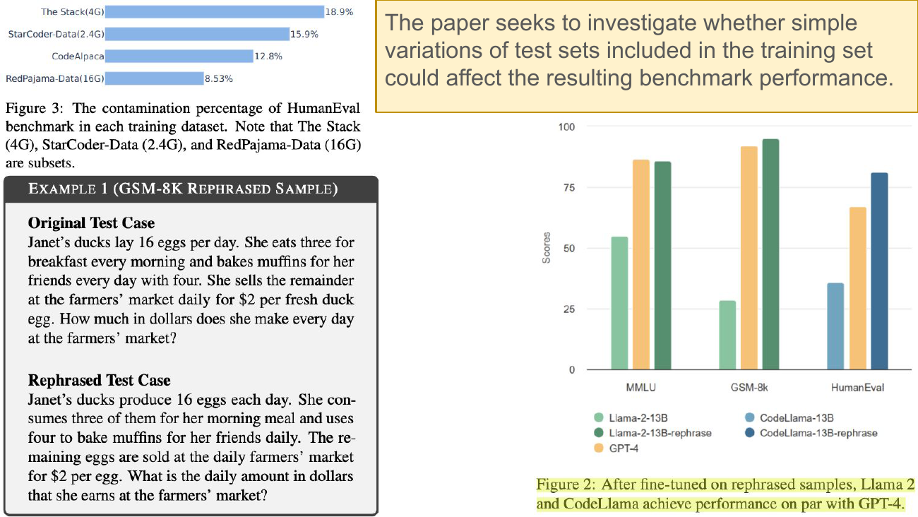
On the slide

Two evidence panels. Top-left: contamination percentages of HumanEval already present in widely-used code datasets (The Stack: 18.9%, StarCoder-Data: 15.9%, CodeAlpaca: 12.8%). Bottom-left: a side-by-side of an original GSM-8K problem and a rephrased version — same problem, different words. Right: after fine-tuning on rephrased samples, Llama-2-13B and CodeLlama-13B match or exceed GPT-4 on MMLU, GSM-8k, and HumanEval.

What to take from it

Contamination isn't a hypothetical risk — it's a documented feature of currently-shipping datasets. Nearly 20% of HumanEval is already in The Stack. Any code model trained on The Stack without proper decontamination is scoring HumanEval partly by recall, not by generalisation.

Slide 30 / 34

LLM Decontaminator. A Venn-like diagram shows Training Data (grey) containing Possible Contamination (light red) which contains Rephrased Samples (dark red). N-gram Overlap catches only a narrow slice, Embedding Similarity Search catches a broad noisy slice (dashed outline), LLM Decontaminator targets the rephrased-samples region precisely. Yellow note: embedding similarity search detects broadly with many false positives; n-gram overlap has limited ability to spot rephrased samples. Bottom-left explains the two-step method: for each test case, identify top-k training items via embedding similarity search, then use an advanced LLM (GPT-4) to judge whether each pair is the same, with a structured prompt asking LLMDetector to return True/False. Right: Algorithm 2 pseudocode for Decontaminate(TrainSet, TestSet, k, Template).

slide 30 · the LLM decontaminator as the proposed fix

On the slide

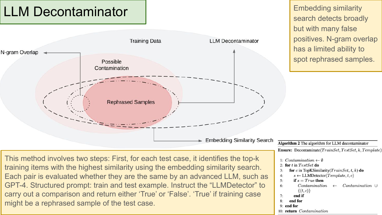
The fix, in two steps. (1) For each test item, use embedding similarity to shortlist the top-k most-similar training items — this is fast and broad. (2) Prompt a strong LLM ("LLMDetector", GPT-4 in the paper) to judge each (train, test) pair: "is this train item a rephrasing of the test item?". Structured prompt, boolean output. Everything flagged True gets removed from the training set.

Why the two-stage design

You can't afford to send every (train, test) pair to GPT-4 — the training set is billions of items. So embedding similarity acts as the coarse retriever (find candidate matches cheaply), and the LLM acts as the precise verifier (judge only the shortlist). This is the same "cheap-retriever + expensive-reranker" pattern that shows up in RAG and in modern search stacks.

⚠ Watch out

This works but doesn't scale. Slide 33 will make the point explicitly: even embedding-shortlisting over a trillion-token corpus is feasible, but LLM-judging every retrieved candidate against every benchmark item costs real money. Semantic decontamination hasn't become the industry default yet because nobody wants to pay for it.

Slide 31 / 34

A table of Training Set, Benchmark, Train/Test size, Rephrased Samples count, and Percentage. Rows include The Stack (4G subset) vs HumanEval 18.9%, StarCoder-Data (2.4G) 15.9%, CodeExercise-Python 15.9%, CodeAlpaca 12.8%, RedPajama-Data-1T (16G) 8.5%, Evol-Instruct-Code 7.9%, rossetacode 2.4%, MATHInstruct vs MATH Test 15.4%, MATH Train 1.6%, FLAN CoT vs MMLU 0.5%, WizardLM-Evol-Instruct vs MMLU 0.5%. Yellow note references related work on temporal leakage in LLM backtesting for stock sentiment signal generation.

slide 31 · contamination table across popular datasets

On the slide

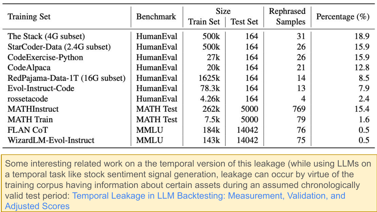
The systematic contamination audit as a table. Reading the rows: over 15% of MATHInstruct rephrases items in the MATH test set. Nearly 19% of The Stack rephrases items in HumanEval. Even instruction-tuned datasets you might have assumed were clean (Evol-Instruct-Code, WizardLM-Evol-Instruct) show non-trivial contamination.

What to take from it

The percentages look small in some rows (0.5% on MMLU) but the absolute numbers are meaningful, and they represent the detectable rephrasings — the true rate is a lower bound. The temporal leakage note in the yellow box is a pointer to Dev et al. 2026, which shows the same problem in a different flavour: benchmarks that involve time-dependent information can leak via the model's knowledge of events that happened during the "test period".

Slide 32 / 34

Other Evaluation Methods: Short Notes. Data Faithfulness — ground-truth comparison (automatic scoring where reference labels exist), human evaluation (accuracy scales with sample size, so does cost), auxiliary model evaluation (model replaces expert, cheaper broader coverage), information extraction (pull relevant spans first so the judge fits them in context). Data Diversity — vocabulary statistics (vocabulary size, n-gram frequency; intuitive but semantically blind), sample relevance (cosine similarity, sample distance; captures semantic spread). Bottom: taxonomy diagram of Direct Evaluation branching into Data Faithfulness (Benchmark, Human, Auxiliary Model Evaluation) and Data Diversity (Vocabulary Statistics, Sample Relevance).

slide 32 · the other half of evaluation, briefly

On the slide

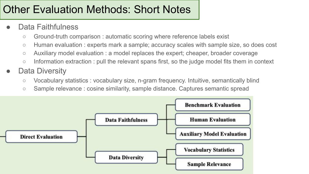
The other things people mean by "evaluation" of synthetic data. Faithfulness gets four sub-methods: ground-truth comparison, human evaluation, auxiliary-model evaluation ("LLM-as-a-judge"), and information extraction. Diversity gets two: vocabulary statistics (n-gram frequency, vocabulary size) and sample-relevance metrics (cosine similarity between samples).

What to take from it

Notice the recurring split: faithfulness and diversity, exactly the two properties introduced back on slide 4. The full loop is: define the two properties, design a pipeline that trades them off, and then use these methods to measure whether the trade-off you picked is the one you actually got. Vocabulary statistics are cheap but blind — "cat cat cat cat" has the same vocab-size score as "cat dog bird mouse". Sample-relevance methods are more expensive but catch semantic collapse.

§9Open problems & bibliography.

The last two slides collect the honest unknowns and the paper list. Read the open problems as an invitation — most of these are wide open and any of them would be a reasonable starting point for a project.

Slide 33 / 34

Open Problems. 1. Semantic decontamination doesn't scale: an embedding index over a trillion-token corpus is affordable, but LLM-judging every retrieved candidate against every benchmark item is not. 2. A bigger teacher doesn't make better data: contrary to expectation, scaling the generator doesn't monotonically help — 8B generators consistently beat 3B ones, but going up to 70B often produced worse synthetic data. 3. No scaling law for synthetic data, and the literature disagrees on the mixing ratio: a 1000-model study found optimal ratios converge near 30% synthetic, stable across sizes and budgets; other 2026 work finds the optimal ratio rises with model size — around 12.5% at 3B and 25% at 6B; WRAP used 1:1; no formal theory yet.

slide 33 · what's actually unsolved

On the slide

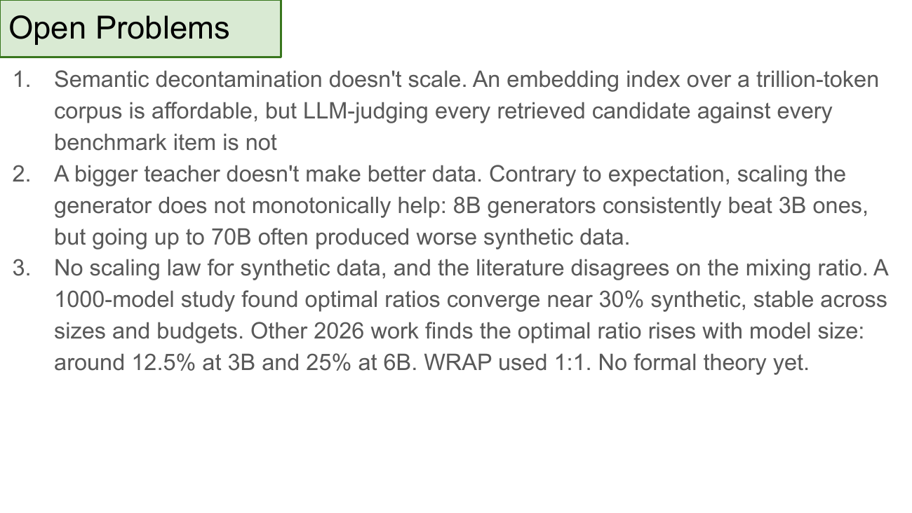
Three concrete open problems:

Semantic decontamination doesn't scale. The LLM-judge approach from slide 30 is the right idea and the wrong cost profile. Someone needs to invent a cheaper semantic matcher, or accept that a small residual contamination rate is the honest baseline.
Bigger teacher ≠ better data. This is a genuinely surprising empirical finding. Naively you'd expect scaling the generator to help monotonically; instead the sweet spot is around 8B for many settings, and 70B generators produce measurably worse data. Nobody has a clean theoretical story for why.
No scaling law for synthetic data. The literature doesn't even agree on the optimal mixing ratio: 30% synthetic (stable across sizes), or a ratio that grows with model size (12.5% at 3B, 25% at 6B), or the 1:1 that WRAP used. All three papers are 2025-26 and disagree.

→ For further reading

All three problems have papers in the bibliography (next slide) pointing at active work. The "generator scale is non-monotone" result is Kang et al. 2025 (arXiv:2510.01631); the mixing-ratio studies are Chen et al. (arXiv:2410.15226) and the 2026 follow-up. Fair game for a project proposal.

Slide 34 / 34

Bibliography. Framework: Long et al., On LLMs-Driven Synthetic Data Generation, Curation and Evaluation: A Survey, ACL 2024, arXiv:2406.15126. Curation: DataComp-LM (Li et al., NeurIPS 2024), FineWeb (Penedo et al., NeurIPS 2024), Broder 1997 SEQUENCES, C4 (Raffel et al., JMLR 2020). Generation — pretraining: WRAP (Maini et al., ACL 2024, arXiv:2401.16380), Nemotron-CC (Su et al., arXiv:2412.02595). Generation — post-training: Self-Instruct (Wang et al., ACL 2023, arXiv:2212.10560), WizardLM/Evol-Instruct (Xu et al., ICLR 2024, arXiv:2304.12244), Stanford Alpaca (Taori et al. 2023). Environments and self-play: Tülu 3 (Lambert et al., arXiv:2411.15124), Absolute Zero (Zhao et al., arXiv:2505.03335), R-Zero (Huang et al., arXiv:2508.05004). Model collapse: Shumailov et al. Nature 2024, Gerstgrasser et al. COLM 2024 (arXiv:2404.01413). Contamination: Yang et al. arXiv:2311.04850, Xu et al. arXiv:2406.04244, Li & Flanigan AAAI 2024, Dev et al. ACL 2026 (Test of Time), LiveCodeBench Jain et al. ICLR 2025, Singh et al. Leaderboard Illusion 2025. Open problems: Nait Saada et al. arXiv:2510.00866, Klimaszewski et al. 2026 (arXiv:2605.23721), Kang et al. EMNLP 2025 (arXiv:2510.01631), Chen et al. arXiv:2410.15226, Zhu et al. DCScore arXiv:2502.08512.

slide 34 · bibliography

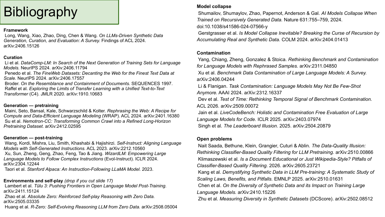
On the slide

The full paper list, grouped by section. Framework (Long et al.), curation (DCLM, FineWeb, Broder, C4), pretraining synthesis (WRAP, Nemotron-CC), post-training synthesis (Self-Instruct, WizardLM, Alpaca), environments and self-play (Tülu 3, Absolute Zero, R-Zero), model collapse (Shumailov, Gerstgrasser), contamination (Yang, Xu, Li & Flanigan, Dev, Jain, Singh), open problems (Nait Saada, Klimaszewski, Kang, Chen, Zhu).

What to take from it

Nearly every entry is from 2023–2026. The field's own literature is younger than the transformers you build models with — most of the papers on this slide didn't exist when GPT-3 was released. Data creation as a distinct research area is genuinely new. That means it's under-explored (good), and also that the "canonical" answer to almost any question you ask hasn't been written yet (also good, from a project-picking perspective).

Zoom out. Data creation splits three ways: curate what already exists, synthesise what doesn't, evaluate whether it actually worked. Curation is subtractive design and it throws away 98% of what it starts with. Synthesis works when a stronger teacher writes for a weaker student, but breaks when you recurse — unless you accumulate instead of replace. Evaluation is the honest step and the one nobody's incentivised to do properly. Every one of these three has open problems with no consensus answers yet. This was a survey pass, not a canonical reference — read Vishal's bibliography for the primary sources.