Lecture 02 · 90 slides · August 3 & 6, 2026

Transformers: the architecture the field lives on.

This deck builds up to the full transformer from the basics: word representations, derivatives, backpropagation, RNN limitations, attention, position, residual paths, normalization, and training. By the end, the goal is not to recognise the Attention Is All You Need diagram, but to understand why each part is there.

Lecture 02 90 slides Aparajitha Allamraju · Manish Shrivastava

§0The deck at a glance

The lecture moves from embeddings and gradients to RNNs, attention, multi-head attention, positional encodings, encoder-decoder models, and training details such as losses, optimizers, and normalization. Treat it as a connected argument for the transformer, not a list of components to memorize.

§1Admin recap

Three quick slides that repeat what Lecture 1 covered: the title card, the seminar rule, the project rule. Nothing new; the instructor wants a stray reminder for anyone who missed day one.

Slide 01 / 90

Title slide: Transformers - Intro, Advanced NLP M26, Aparajitha + Manish Shrivastava, August 3 6 2026, IIIT Hyderabad

slide 01 · title

On the slide

Lecture 2 title card, Transformers, Intro, delivered across two class days, 3 and 6 August 2026, by Aparajitha Allamraju and Manish Shrivastava.

What it means

"Intro" is misleading. This is a 90-slide crash course covering everything from the definition of a derivative to a full encoder-decoder transformer. The reason it is labelled "intro" is that the rest of the course, nine lectures of transformer internals plus everything after, assumes you carry this deck in your head.

Slide 02 / 90

Seminar 10 percent: replaces one exam, not more than 16 approved students, thorough topic presentation not a single paper, evaluated on understanding, coverage, presentation and Q&A.

slide 02 · seminar

Slide 03 / 90

Project 50 percent: propose custom projects, team size 3 or 4, random team allotment available, resubmit if rejected, use TA office hours, compute cannot be provided.

slide 03 · project

On these slides

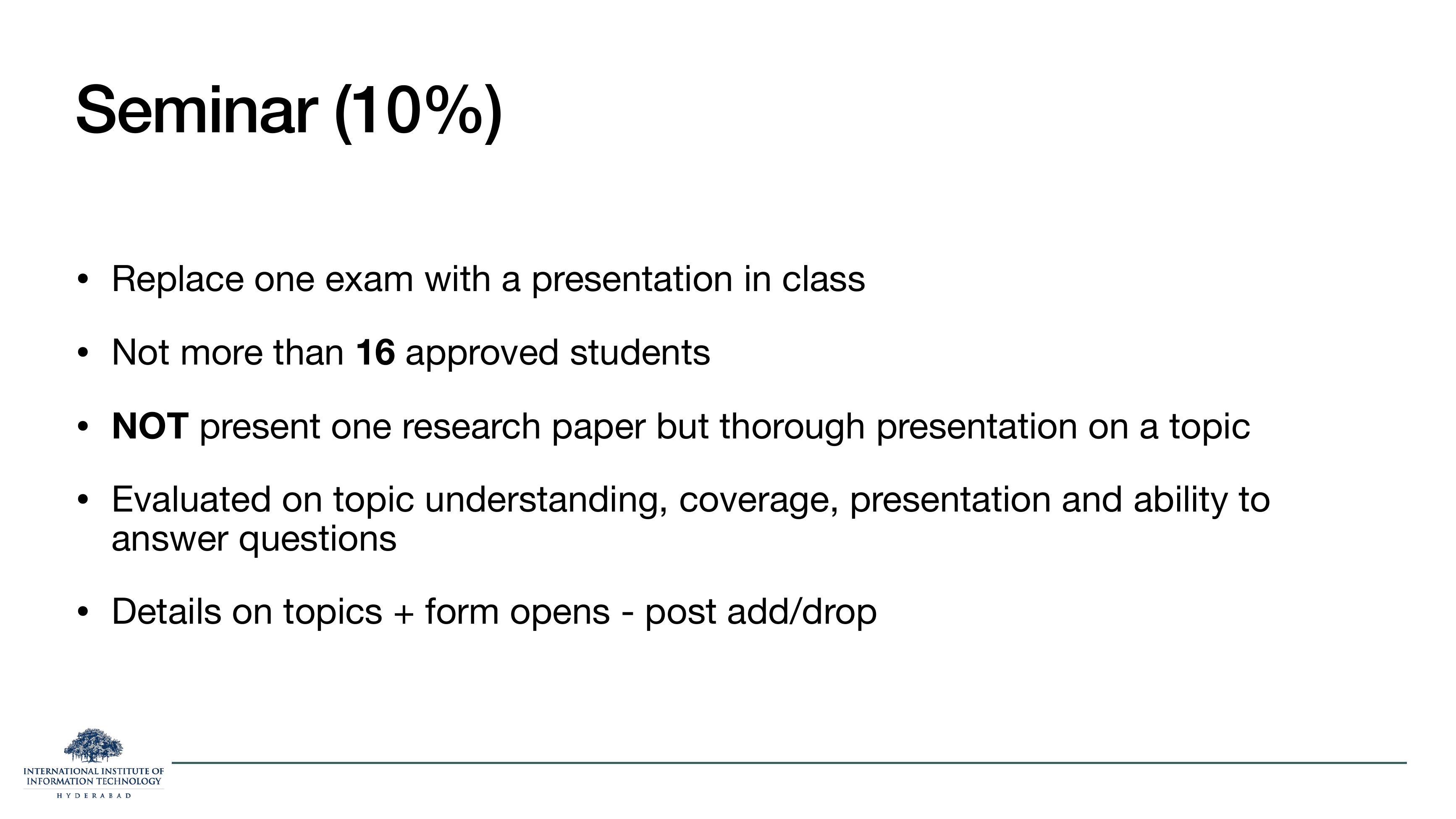
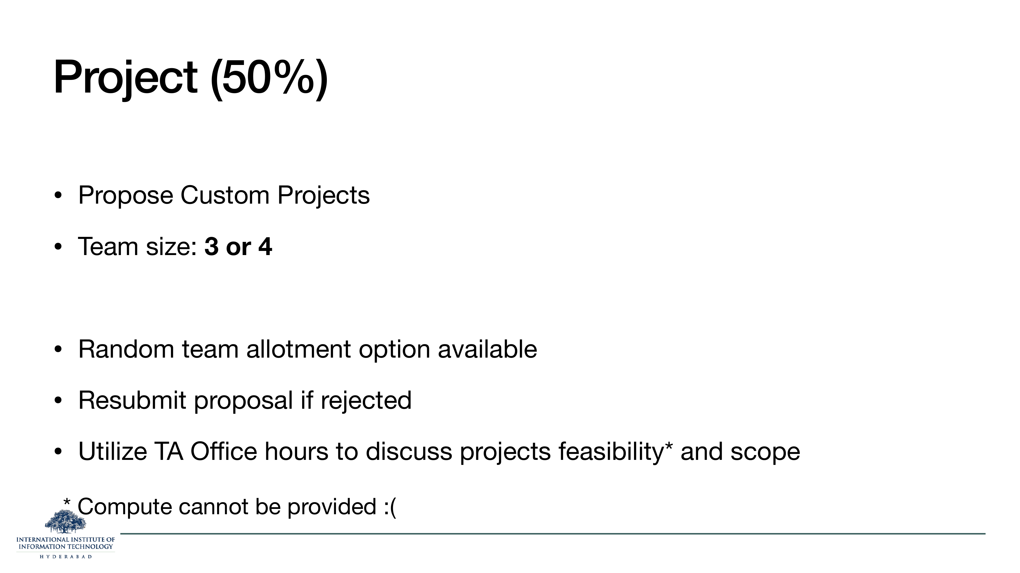
Two administrative reruns from Lecture 1, the seminar option (worth 10%, up to 16 students, replaces one exam) and the project rules (50% of the grade, teams of 3 or 4, no institute compute). See §4 and §5 of Lecture 1 for the full breakdown.

Why it is here again

The instructor knows some students only turn up from Lecture 2 onwards. Anything that costs marks gets repeated in the second lecture as a courtesy.

→ Keep reading

Cross-reference: full logistics in Lecture 1.

§2Word representations, in one page

The lecture opens the technical content with a Recap divider and then one big slide summarising the evolution of word representations. This is fifteen years of NLP compressed into five bullets, so the density is deceptive. It is worth reading slowly.

Slide 04 / 90

slide 04 · section divider

A one-word section divider. Everything until slide 12 or so is background you might already have, taught fast for anyone who does not.

Slide 05 / 90

Word Representations Evolution: one-hot vector, tf-idf, Word2Vec/GloVe/fasttext, BERT, LLM embeddings. As you go down the list, Context goes Low to High, Ambiguity High to Low, Sparsity Sparse to Dense, Complexity Low to High.

slide 05 · evolution of embeddings

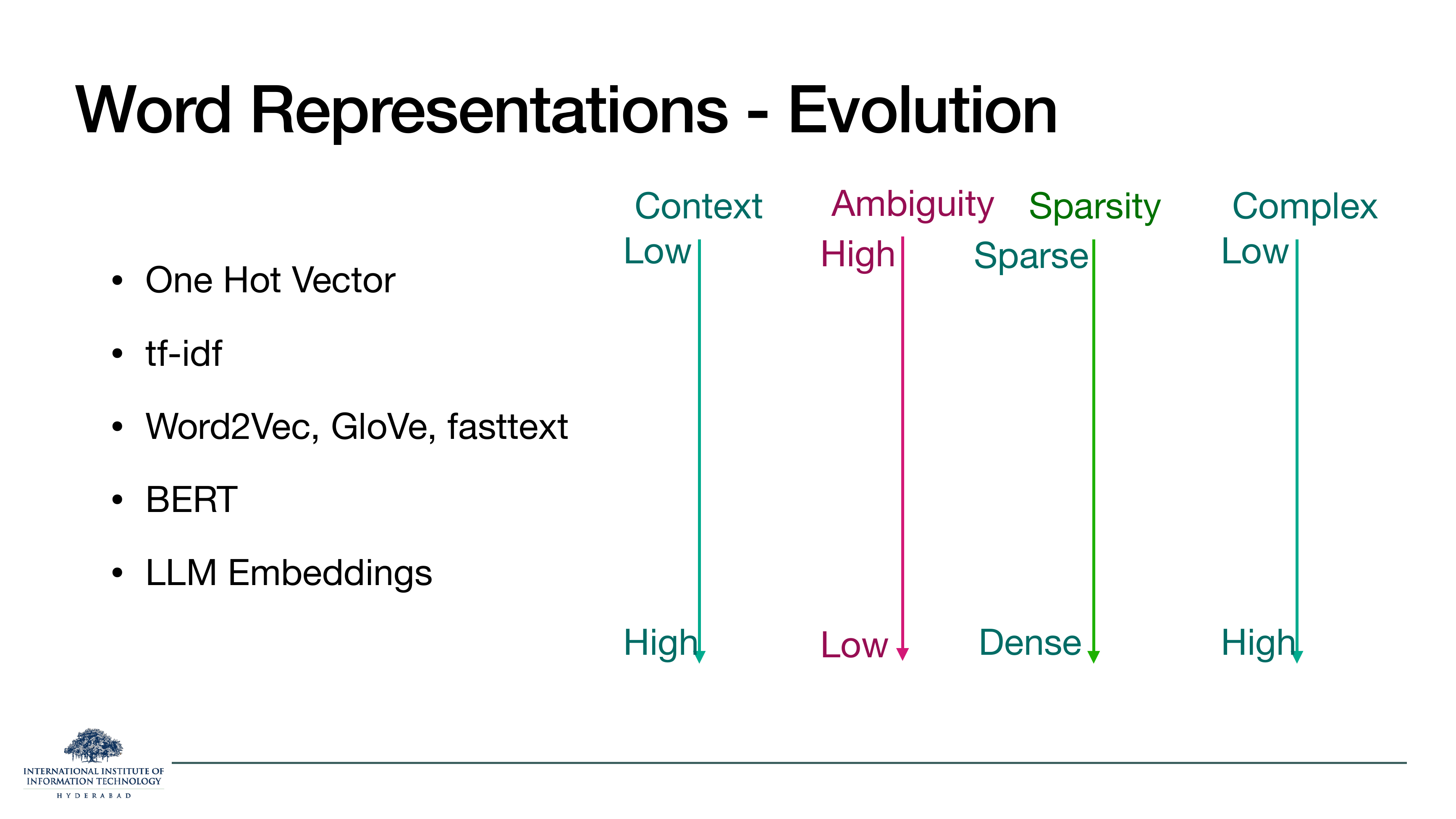
On the slide

Five ways to represent a word, ordered oldest to newest, with four axes on the right that shift as you descend the list.

One-hot vector. A vector as long as the vocabulary, all zeros except a single 1 at the word's index. No context, maximum sparsity, maximum ambiguity (every sense of "bank" gets the same vector).
tf-idf. Term frequency scaled by how rare the word is in the corpus. Still sparse, still context-free, but at least common words like "the" carry less weight.
Word2Vec, GloVe, fastText. Dense vectors (typically 100 to 300 dimensions) learned so that words in similar contexts get similar vectors. Still one vector per word type, "bank" (river) and "bank" (finance) collapse.
BERT. The vector for a word depends on its sentence. Two different uses of "bank" now get two different vectors.
LLM embeddings. Same idea, bigger models, and the vectors are learned end-to-end on next-token prediction over web-scale text.

✦ Key takeaway

Read the four arrows on the right of the slide together. As we move down the list, representations get more contextual, less ambiguous, more dense, and more complex to train. Every step of the evolution buys context by paying complexity. That trade is the through-line of the whole course.

→ Keep reading

Lecture 3 on Tokenization zooms into the "what is a word" question this slide silently assumes. The Embeddings lecture zooms into Word2Vec / GloVe / fastText themselves.

§3Gradients & backprop, from scratch

Ten slides of calculus. The lecturer is not being nostalgic. Everything in the rest of the deck, every architectural choice, every normalisation trick, is motivated by how gradients flow through the network. If you cannot picture a gradient moving backwards through a matrix multiply, the transformer diagram will feel arbitrary. Read this section as the answer to the question "why does anything need to be added to a plain matrix multiply".

Slide 06 / 90

slide 06 · section divider

Section divider. From here through slide 15 the lecture rebuilds calculus, one derivative at a time, up to the operations you actually run inside PyTorch.

Slide 07 / 90

Gradients slide: gradient is slope, derivative of a function; change in output wrt change in input; example f(x)=x^n, f'(x)=nx^(n-1).

slide 07 · derivative

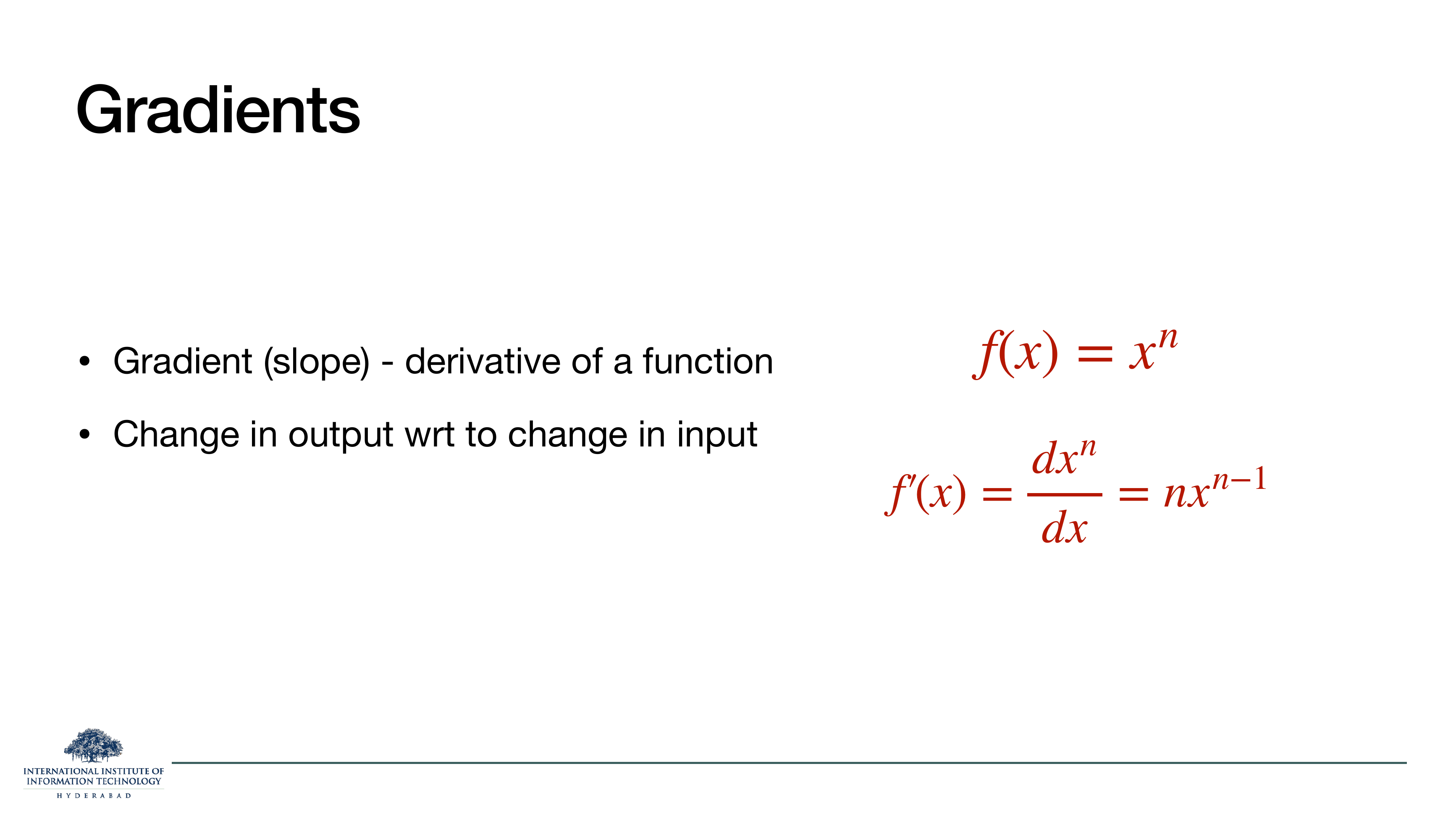
On the slide

A one-line definition: the gradient is the derivative of a function, the change in its output per unit change in its input.

What it means

For a scalar function like f(x) = xⁿ, the derivative f'(x) = n x^n-1 tells you the slope at any point. In a neural network the "function" is the loss and the "input" is a parameter. So the gradient answers: if I nudge this weight by a tiny amount, does the loss go up or down, and by how much?

Under the hood

Every training step is: (1) evaluate the loss, (2) compute the gradient of the loss with respect to every parameter, (3) move each parameter a small step downhill. The rest of this section is the machinery for step 2.

Slide 08 / 90

Gradients: function with 1 output and n inputs. f: R^n -> R. Gradient is a vector of partial derivatives ∂f/∂x_1, ..., ∂f/∂x_n.

slide 08 · gradient vector

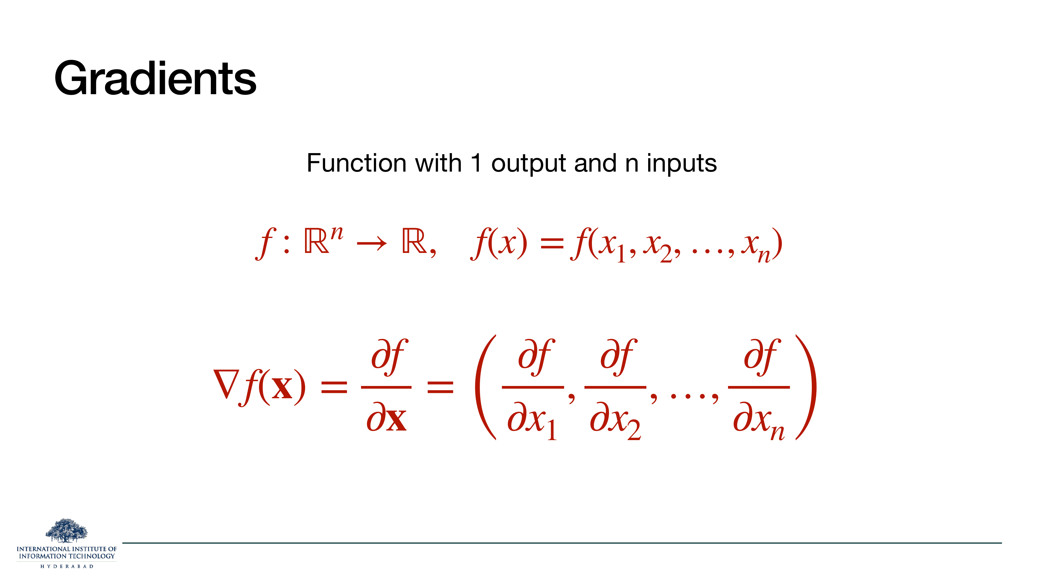
On the slide

Same idea, but for functions of many variables. If f takes n inputs and returns one number, its gradient ∇f(x) is the vector of all n partial derivatives.

What it means

A neural network's loss depends on millions of parameters. The gradient is a vector of the same shape as your parameters: one number per weight, saying which way to push that weight. Gradient descent is literally "subtract a small multiple of this vector from your parameters".

Slide 09 / 90

Jacobian Matrix: function with m outputs and n inputs. f: R^n -> R^m. Jacobian is the m-by-n matrix of all partial derivatives ∂f_i/∂x_j.

slide 09 · Jacobian

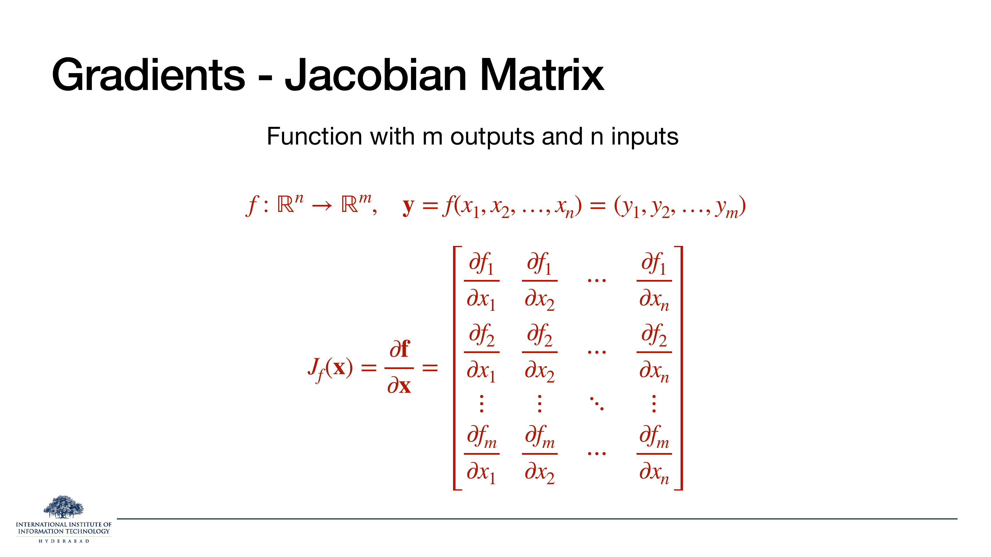
On the slide

Now the function has many inputs and many outputs. The Jacobian J_f(x) is the m×n matrix whose (i,j) entry is the partial derivative of the i-th output with respect to the j-th input.

Why keep this in mind

Every layer of a neural network is a function from vectors to vectors. So its "gradient" is a Jacobian. Backpropagation is nothing more than repeatedly multiplying these Jacobians together via the chain rule, only, because the final output is a single scalar (the loss), the whole chain collapses back into a gradient vector at the end.

Slide 10 / 90

Hessian Matrix: second-order partial derivatives of a scalar-valued function. H_f(x) = ∇²f(x), an n-by-n matrix.

slide 10 · Hessian

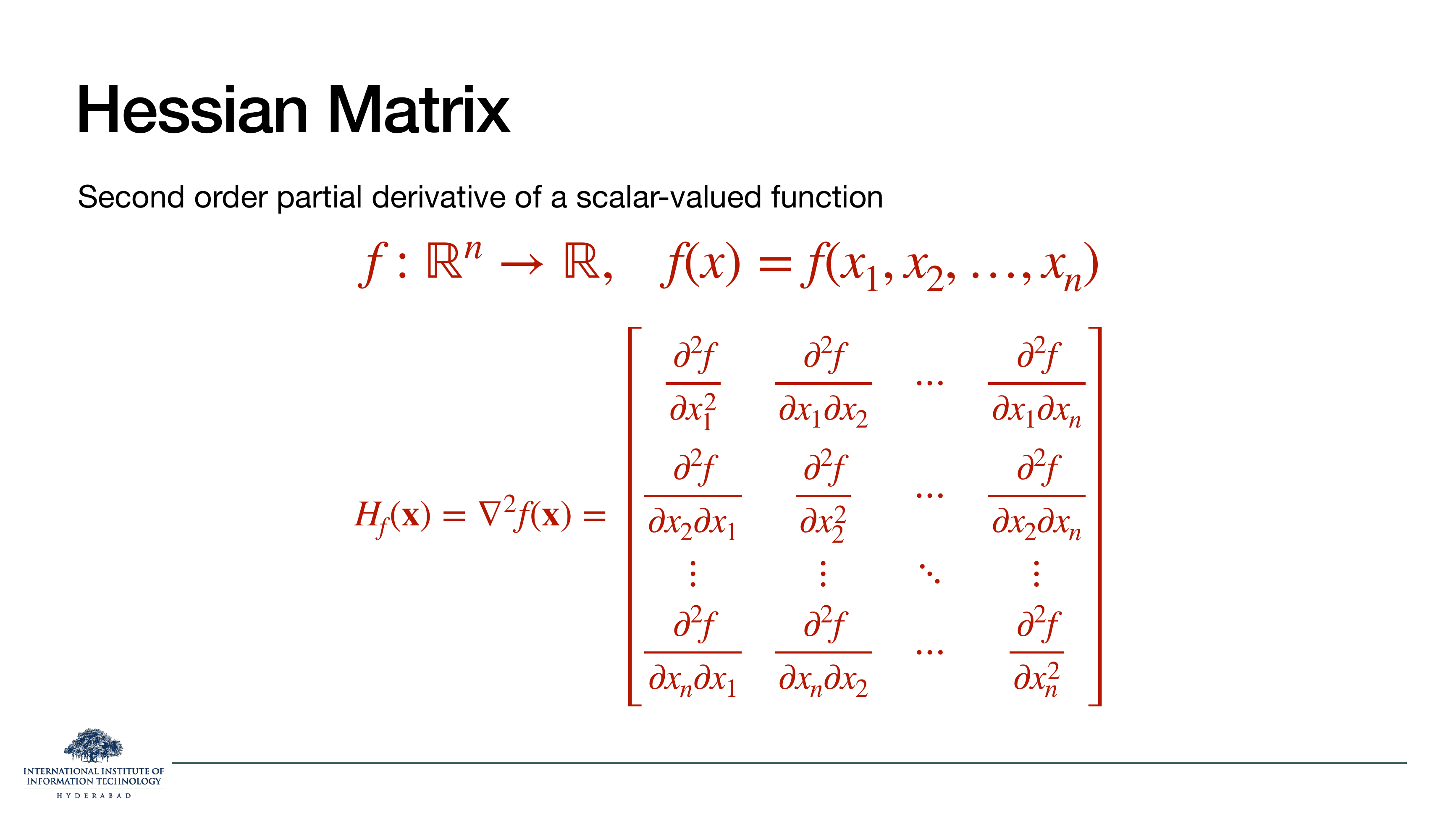
On the slide

The Hessian is the matrix of second partial derivatives. It tells you not just the slope but the curvature of the loss surface.

Why it matters in practice

Newton's method uses the Hessian to pick step sizes automatically. Modern deep learning almost never does this: a Hessian for a billion-parameter model is a billion-by-billion matrix, and just storing it is impossible. What optimisers like Adam do instead is estimate a cheap proxy for curvature from the running mean and variance of the gradient itself. But the Hessian is worth knowing exists, it is what "second-order optimisation" refers to and what algorithms like L-BFGS approximate.

Slide 11 / 90

Gradient Descent: minimize objective J(θ), random parameter init θ, find slope ∇_θ J(θ), move θ = θ - η ∇_θ J(θ). Adjust model parameters to minimize error.

slide 11 · gradient descent

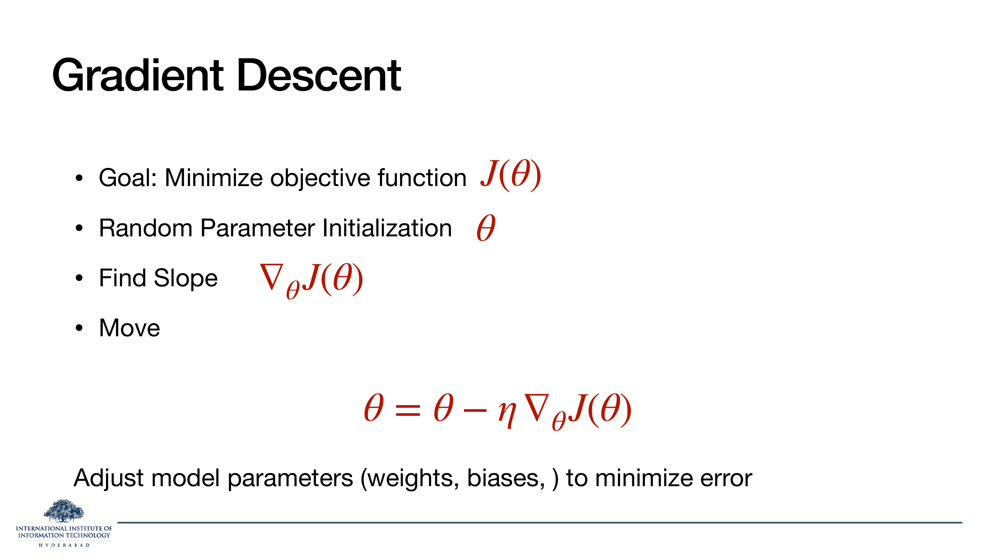
On the slide

The training loop in one equation: θ ← θ − η ∇_θ J(θ). Initialise parameters randomly, compute the gradient of the loss, take a small step in the opposite direction, repeat.

θ \leftarrow θ - η \nabla J (θ)

What it means

The letter η ("eta") is the learning rate, how big a step to take. The letter J is a common name for the loss (older literature used it for the "cost function"; you will more often see L in modern papers). This is the entire recipe for training any model in the course.

Slide 12 / 90

Stochastic Gradient Descent: optimization on traditional GD (which is slow and memory-intensive). Calculate gradients for each training sample or batch instead of full dataset. θ = θ - η ∇_θ J(θ; x_i; y_i).

slide 12 · SGD

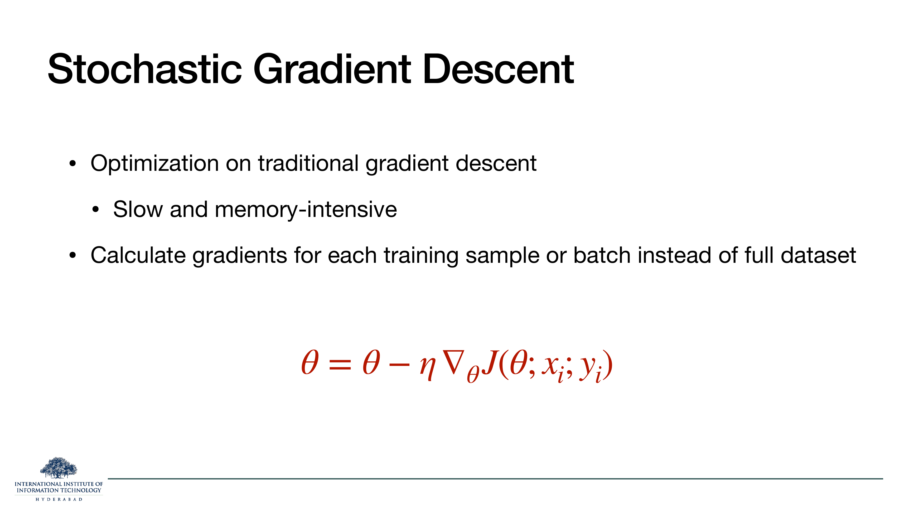
On the slide

The practical version: instead of computing the gradient over the entire dataset (impossible when the dataset is bigger than memory), estimate it from one sample or one mini-batch at a time.

What it means

Full-batch gradient descent is precise but glacial. Stochastic gradient descent (SGD) trades precision for speed: each step is noisy, but you get many, many steps per unit of compute. Every optimiser in the rest of the course, SGD, Adam, AdamW, Lion, is a variant of this idea with a smarter learning rate.

Slide 13 / 90

Gradient Descent vs SGD: SGD zigzags noisily towards the minimum, plain GD walks smoothly to it.

slide 13 · GD vs SGD

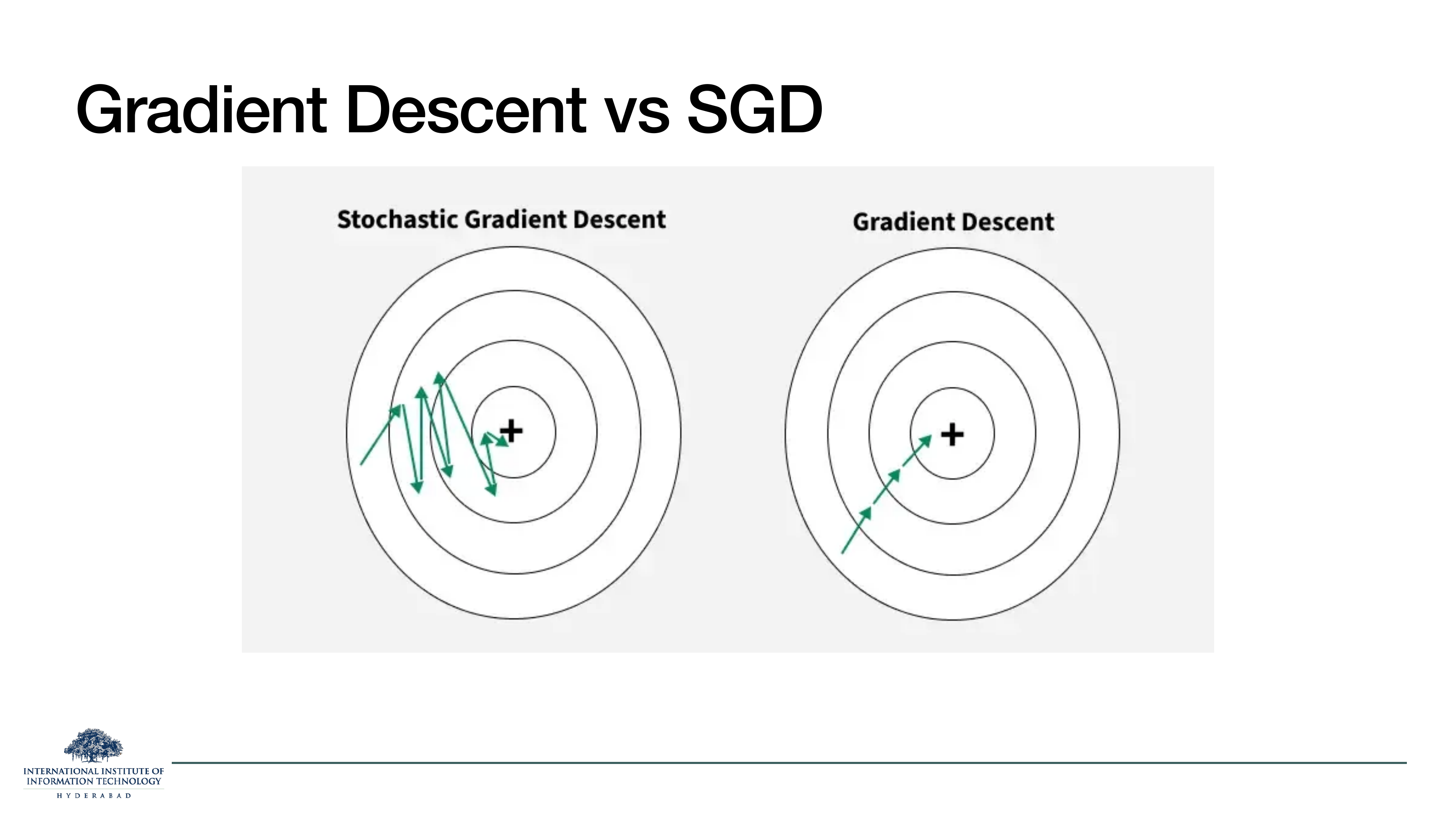
On the slide

Two loss contour plots. On the left, SGD's path zig-zags towards the centre because each step is based on a noisy gradient estimate. On the right, full-batch GD walks smoothly to the minimum.

✦ Key takeaway

The noise in SGD is not just a bug we tolerate for speed. It is a feature: the jitter helps the optimiser escape shallow local minima and saddle points that would trap a smoother trajectory. Deep-learning loss surfaces are full of saddle points; SGD's noise is what lets it keep moving.

Slide 14 / 90

Learning Rate η: step size to descent. Too small: slow convergence. Too big: overshoot.

slide 14 · learning rate

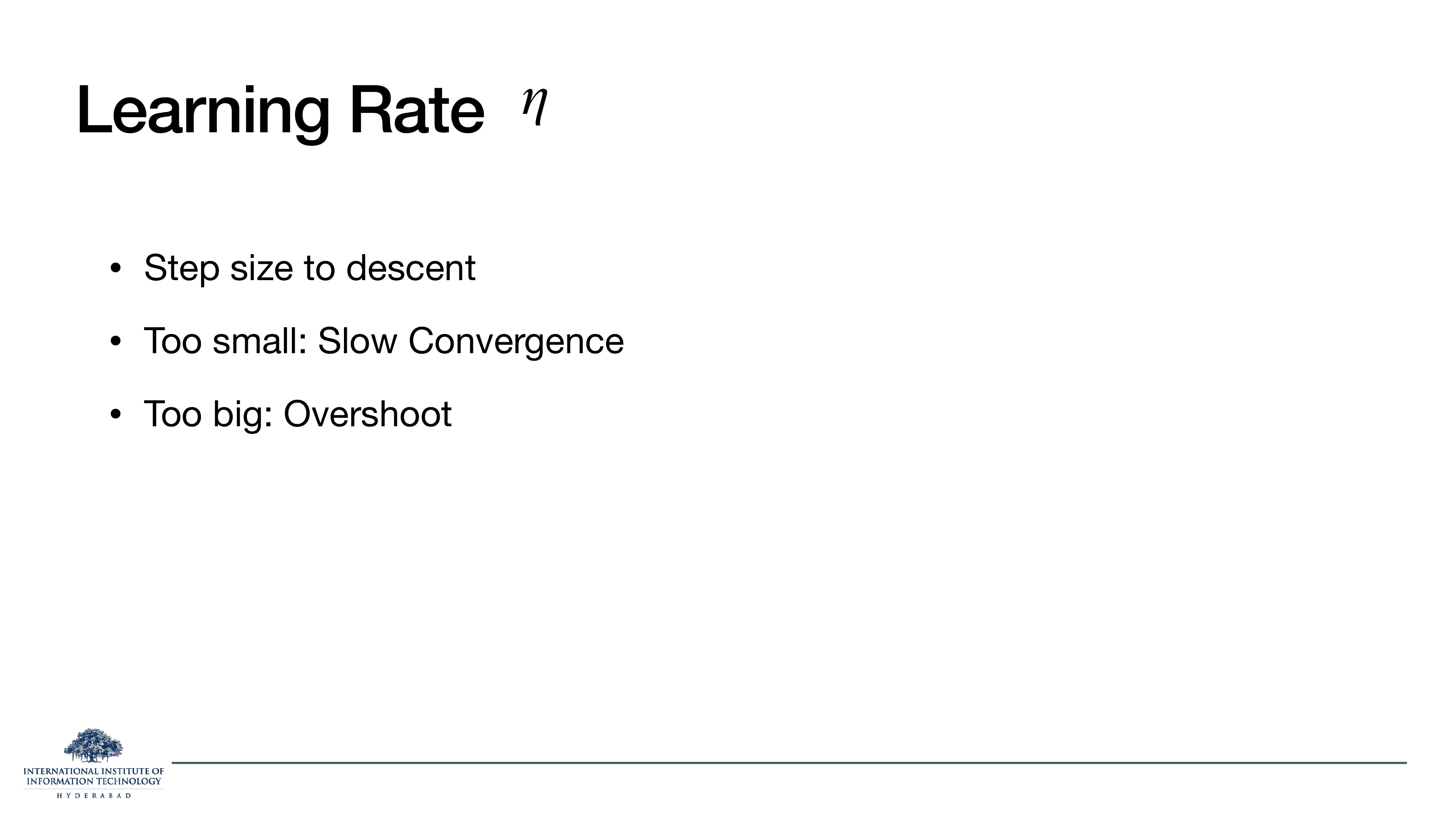
On the slide

The learning-rate trade-off. Too small and the loss barely moves per step; too large and each step overshoots the minimum and can diverge.

What it means

Picking η is one of the single most important knobs in deep learning. For transformers, the standard practice is a warmup + decay schedule: ramp up from zero over a few thousand steps, then decay. We will meet the schedule again in §9.

Slide 15 / 90

Learning Rate Fixes: gradient clipping, weight regularizations, batch normalization.

slide 15 · training fixes

On the slide

Three tricks that let you use a larger, more aggressive learning rate without blowing up.

Gradient clipping caps the norm of the gradient vector, so one anomalous batch cannot send weights to infinity.
Weight regularisation (L1, L2, weight decay) penalises large weights, which keeps the loss surface flatter and better conditioned.
Batch normalisation rescales activations so successive layers see inputs of similar magnitude, a stabiliser we will revisit as layer norm in the transformer.

→ Keep reading

Layer norm and RMSNorm both live inside every transformer block. See §8 for how they wire in.

§4Backpropagation, the picture

Six slides on the mechanic that actually computes those gradients: forward pass, backward pass, then a hand-drawn chain of hidden states that walks the loss gradient right back to the first layer. The last slide in this run, the product of Jacobians, is the seed of the vanishing-gradient problem that will motivate attention two sections later.

Slide 16 / 90

Backpropagation: reduce error by adjusting weights and biases; two phases — forward pass, backward pass.

slide 16 · backprop overview

On the slide

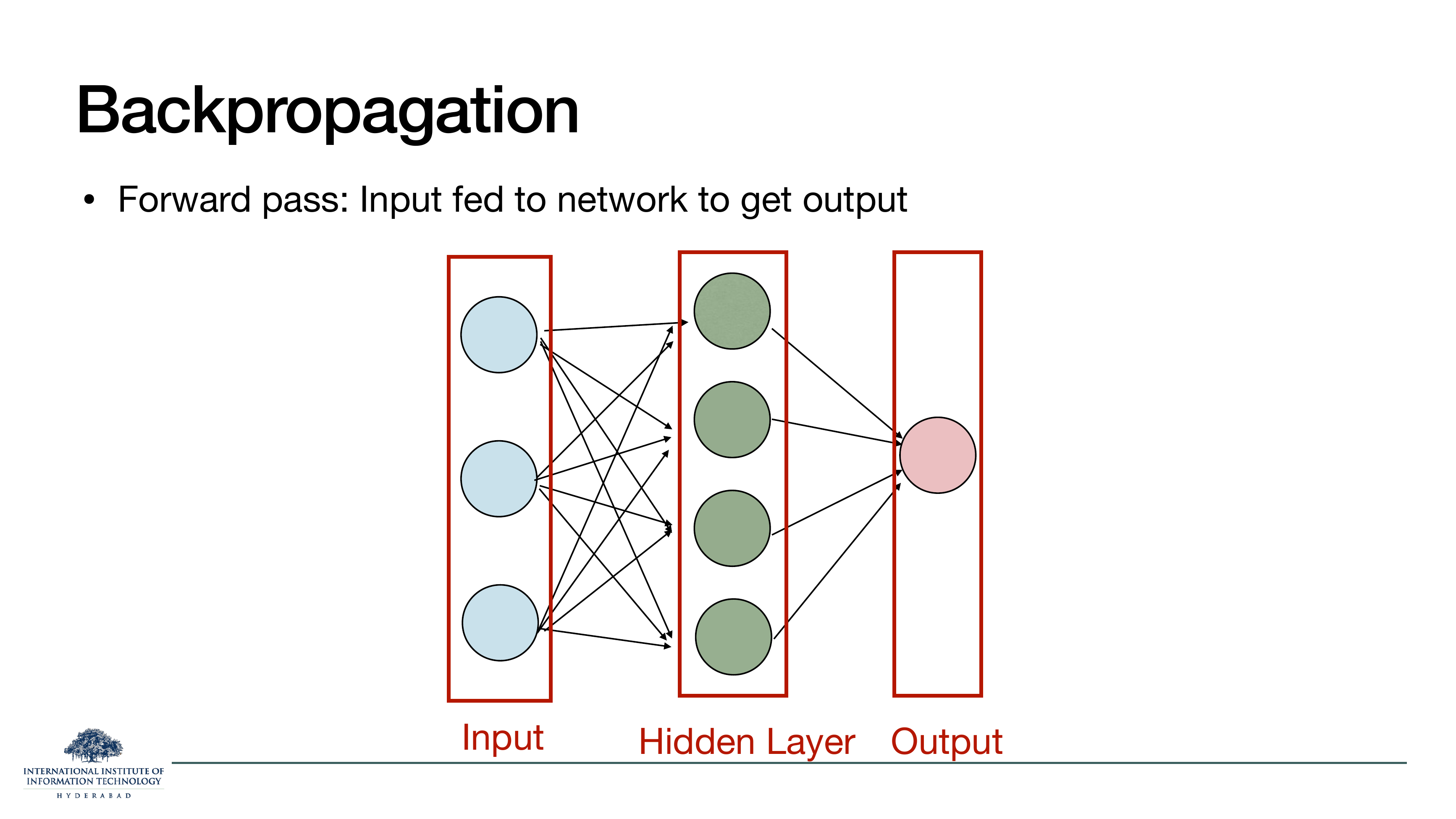
Training a network alternates between a forward pass (feed the input through, compute the loss) and a backward pass (propagate the gradient of the loss back to every parameter).

What it means

Backpropagation is not a new algorithm on top of the chain rule, it is the chain rule, applied to a computation graph in reverse. The name is 40 years old (Rumelhart, Hinton, Williams, 1986); everything since has been engineering.

Slide 17 / 90

Forward pass diagram: input layer of 3 blue nodes, hidden layer of 4 green nodes, and output node in pink; arrows go left to right through all connections.

slide 17 · forward pass

Slide 18 / 90

Backward pass: error calculation, propagation of gradients.

slide 18 · backward pass

On these slides

The two halves of a training step. Forward: multiply the input by the weights layer by layer to produce a prediction. Backward: compute the error (prediction minus target), then propagate that error backwards through the same weights, accumulating a gradient for each parameter along the way.

Under the hood

In PyTorch: the forward pass builds a graph, loss.backward() walks it in reverse and fills in .grad on every tensor. That is literally the API the two slides describe.

Slide 19 / 90

Calculating gradients: a chain of hidden states h1 -> h2 -> h3 -> h4 with the same weight W_h between each pair; a loss L at the end; a red arrow shows gradient ∂L/∂h_1 flowing back from L all the way to h_1.

slide 19 · loss reaches the first layer

On the slide

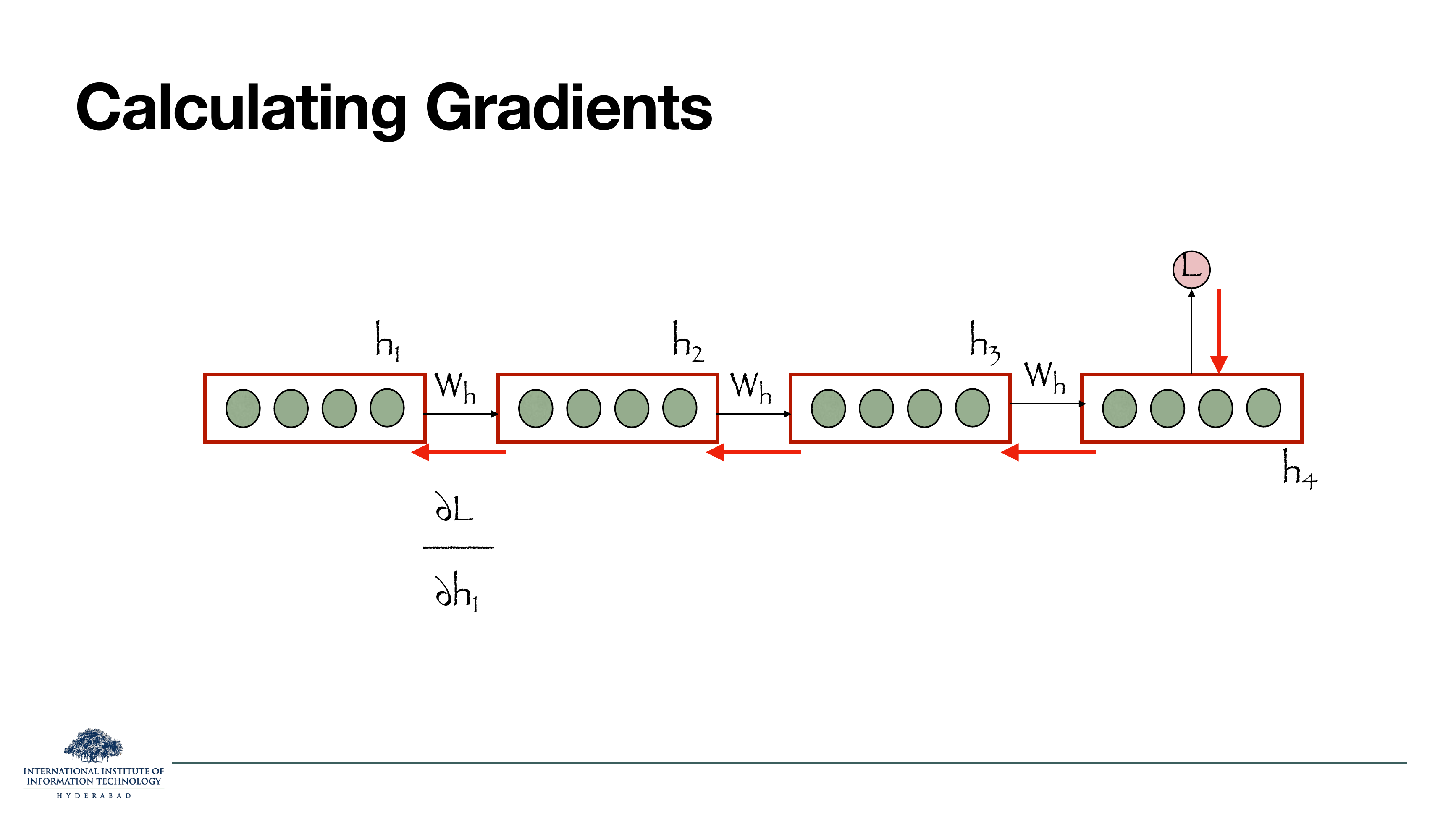
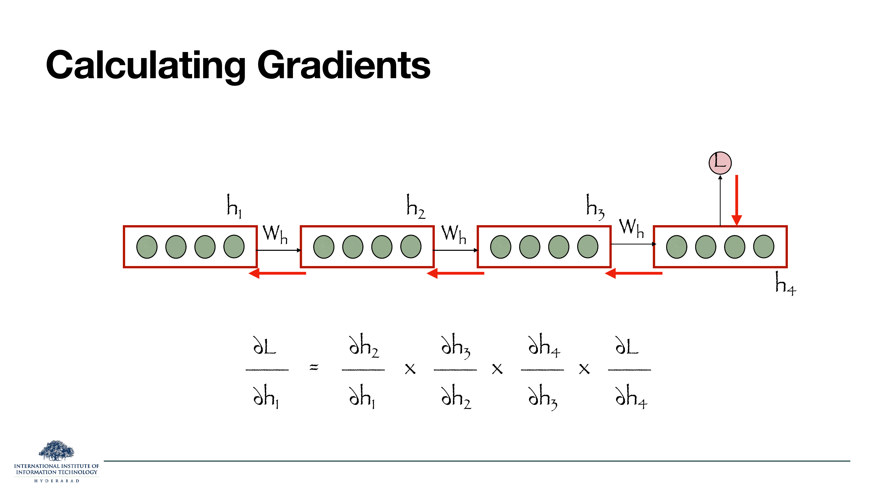
A chain of hidden states h₁, h₂, h₃, h₄ with the same weight matrix W_h between each pair. The loss L sits at the end. The red arrows show the gradient of the loss flowing backwards to h₁.

Why the shared weights matter

Reusing the same W_h across time steps is the picture of a Recurrent Neural Network unrolled. It is also why RNNs have so few parameters compared to their depth, and, as the next slide makes explicit, why they struggle to train.

Slide 20 / 90

Same chain h1..h4 with L at the end; now every intermediate gradient ∂L/∂h_i is labelled.

slide 20 · every gradient labelled

Slide 21 / 90

Same chain, with the chain rule expansion below: ∂L/∂h_1 ≈ (∂h_2/∂h_1) × (∂h_3/∂h_2) × (∂h_4/∂h_3) × (∂L/∂h_4).

slide 21 · chain rule product

On these slides

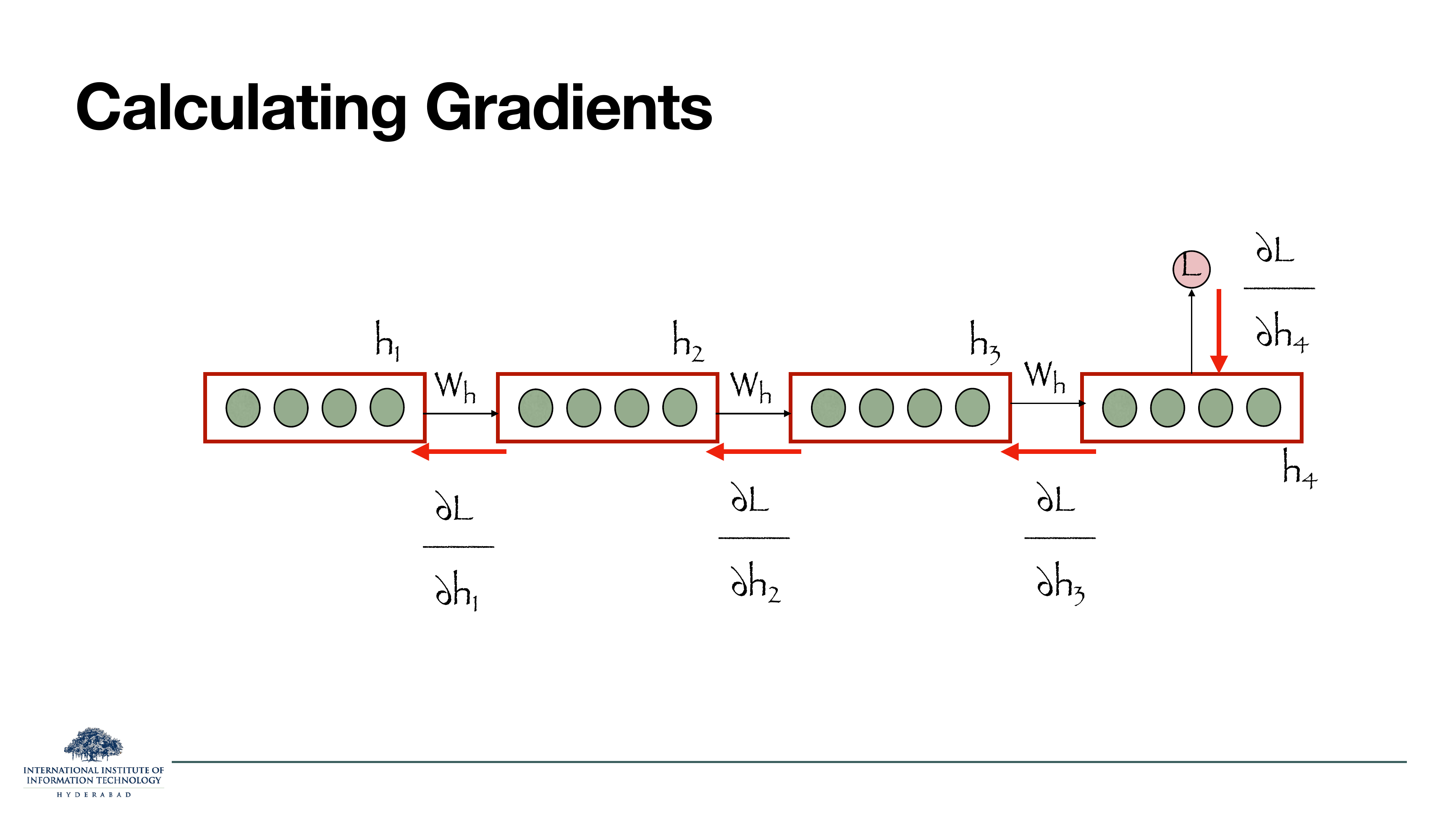
Slide 20 labels every intermediate gradient in the chain. Slide 21 writes out the reason: the gradient at the first layer is the product of all the intermediate Jacobians times the gradient at the loss.

\frac{\partial L}{\partial h_{1}} = \frac{\partial h_{2}}{\partial h_{1}} \times \frac{\partial h_{3}}{\partial h_{2}} \times \frac{\partial h_{4}}{\partial h_{3}} \times \frac{\partial L}{\partial h_{4}}

✦ Key takeaway

Read that formula and ask: what happens if each of those Jacobians has entries smaller than 1? The product shrinks exponentially. If they are larger than 1, it explodes. This is the vanishing / exploding gradient problem, the single reason plain RNNs cannot learn long-range dependencies, and the reason the transformer's shortcut connections were invented. Hold this picture in your head; the entire next section is a reaction to it.

§5Neural nets in NLP, and what broke

Fifteen slides on the pre-transformer world. The lecture uses the RNN as a foil: it walks you through the RNN language model, names the three ways it fails (finite context, long-distance dependency, no parallelism), gives you five kinds of linguistic dependency that break its back, then shows the LSTM as the partial fix that dominated NLP from 2015 to 2017. All of it exists so the next section can say "and then attention just replaced this whole picture".

Slide 22 / 90

slide 22 · section divider

Section divider. From here the lecture stops teaching calculus and starts building the actual neural architectures NLP used before transformers.

Slide 23 / 90

RNN language model: 'The student opened their', each word fed as x_i, embedded via E, projected by W_e into a hidden state which is passed forward with W_h; final hidden state produces a distribution y over the vocabulary — books, laptops most likely.

slide 23 · RNN language model

On the slide

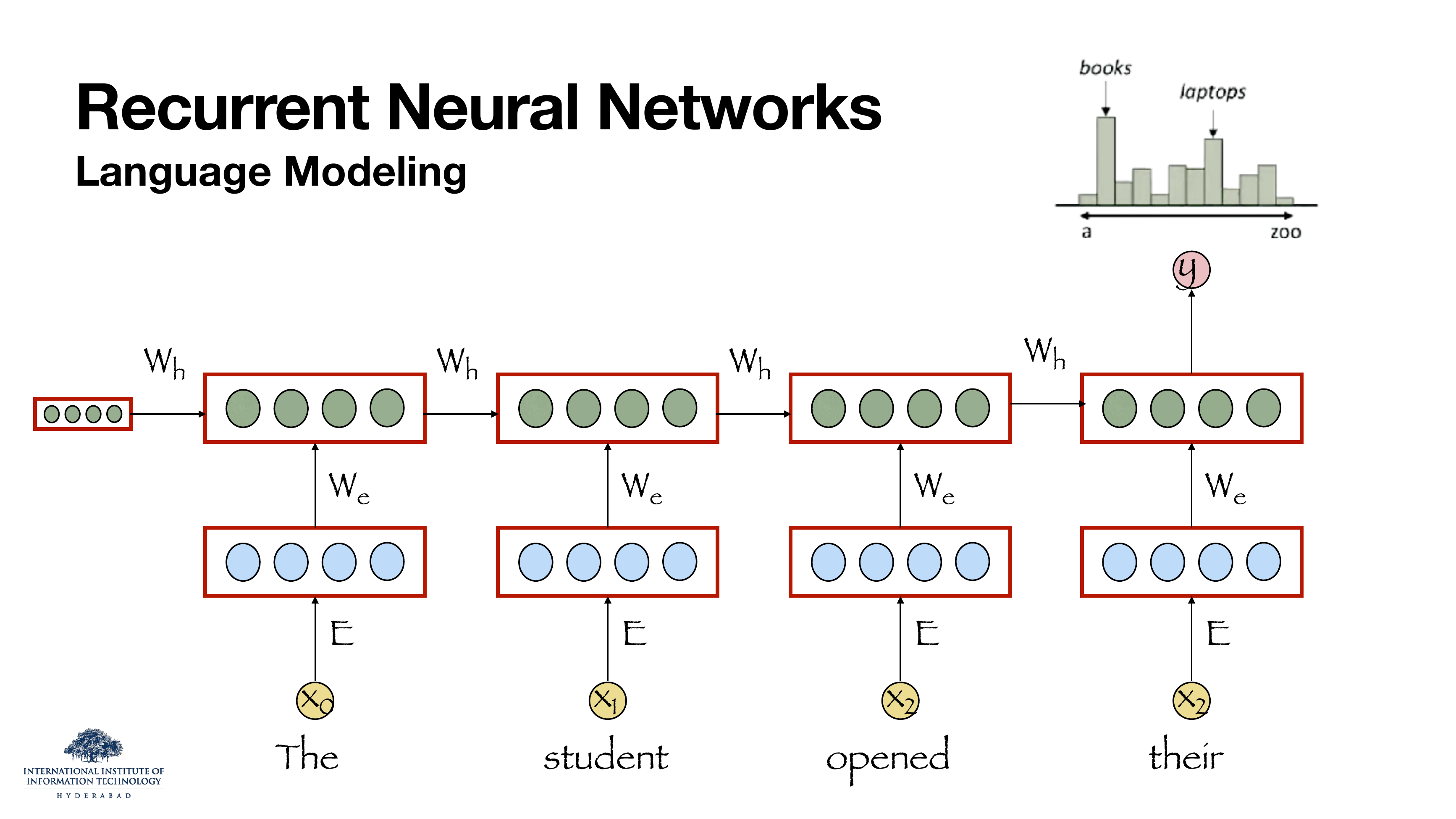
The classic Recurrent Neural Network language model, unrolled over the sentence "The student opened their ___". Each token x_i becomes an embedding via matrix E, is projected by W_e into a hidden state, and combined with the previous hidden state via W_h. The final hidden state produces a distribution y over the next word.

What it means

The whole sentence's context is compressed into one fixed-size hidden vector before you ever predict a word. The same W_h is reused at every step; that is what "recurrent" means. This is elegant and it works, but the next four slides list what it cannot do.

Slide 24 / 90

RNN Limitations: finite context, long distance dependency, lack of parallelizability.

slide 24 · RNN limitations

On the slide

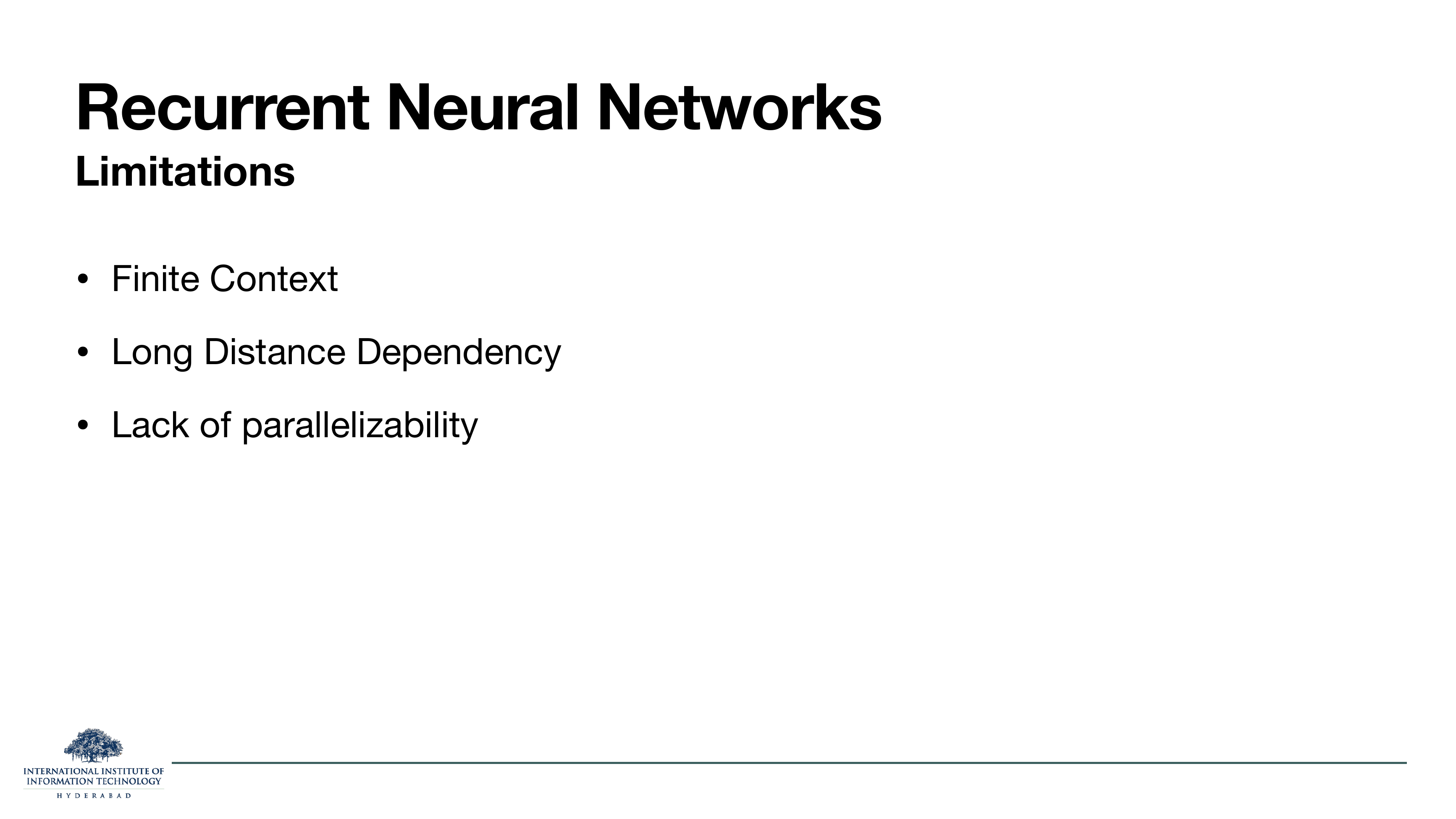
Three fatal weaknesses of the RNN, and every one of them is a headline problem the transformer will need to solve.

Finite context. Everything the model knows about the past is squeezed into one fixed-size vector.
Long-distance dependency. Words far back in the sentence have almost no influence on the current prediction (this is the vanishing gradient again).
Lack of parallelisability. To compute h_t you must first compute h_t-1. A GPU cannot help you here, the recurrence is inherently sequential.

✦ Key takeaway

Item 3 is the one that ends up mattering most. The transformer will accept a bigger parameter count and more FLOPs per token, but it can do them all in parallel. In the GPU era, "trainable in a week" beats "elegant but sequential" every time.

Slide 25 / 90

Vanishing gradient: gradients less than 1 get smaller and smaller; gradient signal from far is lost; model weights updated with only near relations not long-term.

slide 25 · vanishing gradient

Slide 26 / 90

Exploding gradient: gradients much greater than 1, update step too large; rarer than vanishing; can be fixed with gradient clipping.

slide 26 · exploding gradient

On these slides

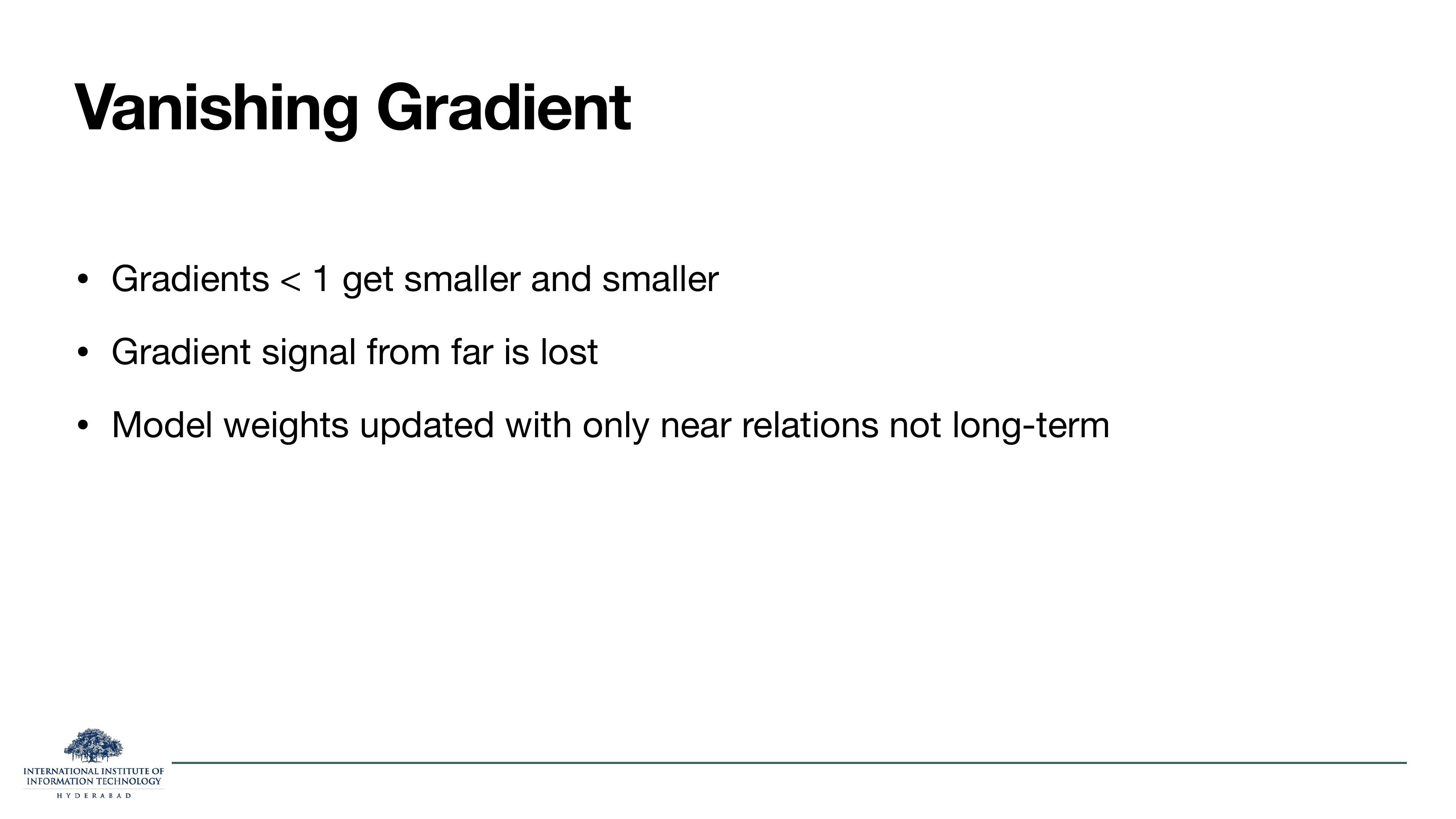
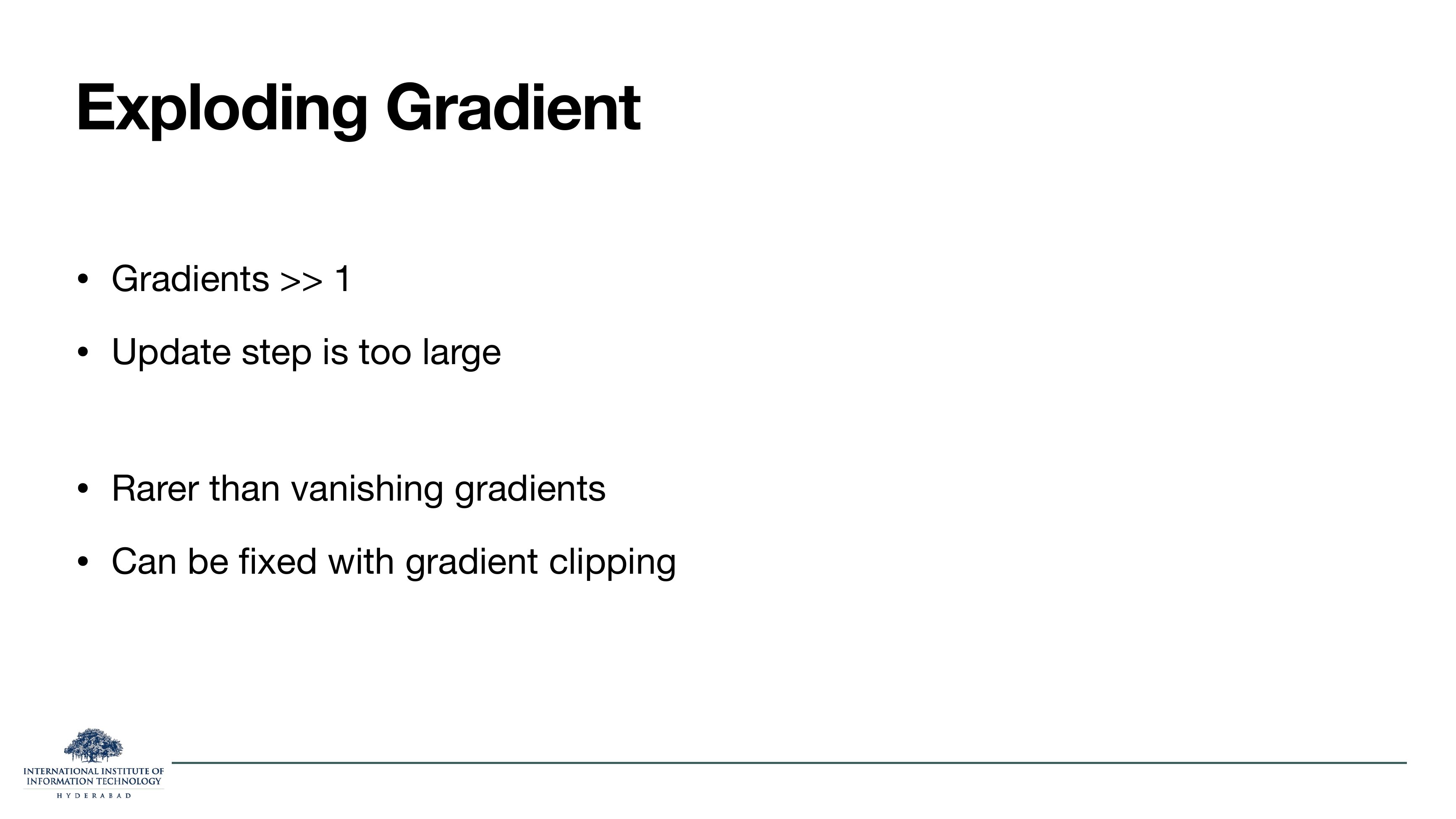
Two sides of the same coin. The product of Jacobians we wrote in §4 is a game of exponents: if factors are smaller than 1 the gradient vanishes to zero, if they are larger than 1 it explodes to infinity.

Consequences

A vanishing gradient means the model can only learn from words a few tokens back, the very long-distance dependencies (slides 33 and 34, coming up) never train. An exploding gradient sends the update step to infinity and blows the loss up. The vanishing case has no cheap fix; the exploding case does, clip the gradient norm at every step.

Slide 27 / 90

Section divider: Long Dependencies in Language

slide 27 · section divider

A brief interlude, five slides on why long-distance dependencies actually matter for language, not just as an abstract complaint about RNNs.

Slide 28 / 90

Relationships in Natural Language: anaphora, co-reference, causal, temporal, discourse structures.

slide 28 · relationships in language

On the slide

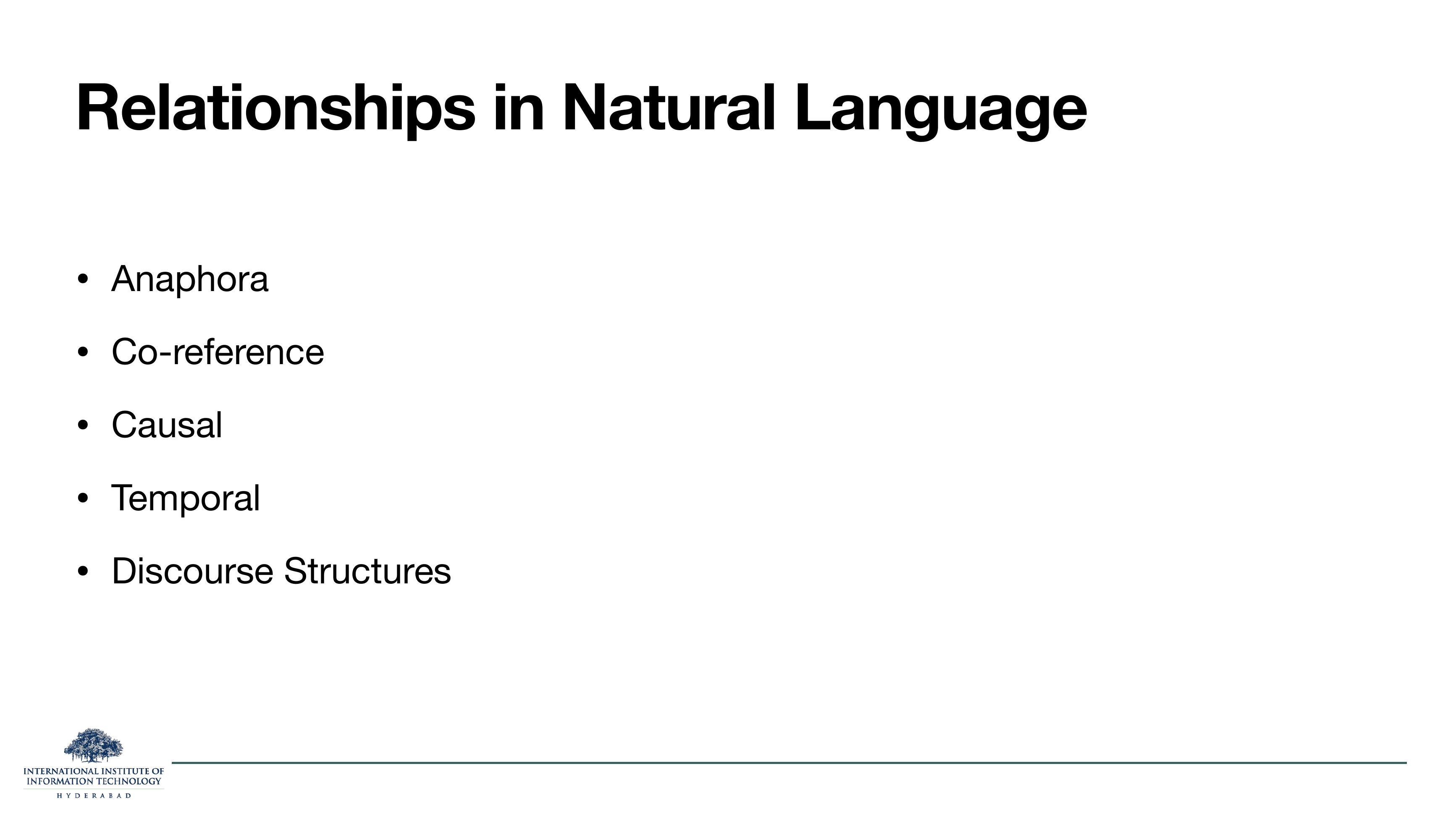
Five kinds of long-range structure that a language model must handle to be any good.

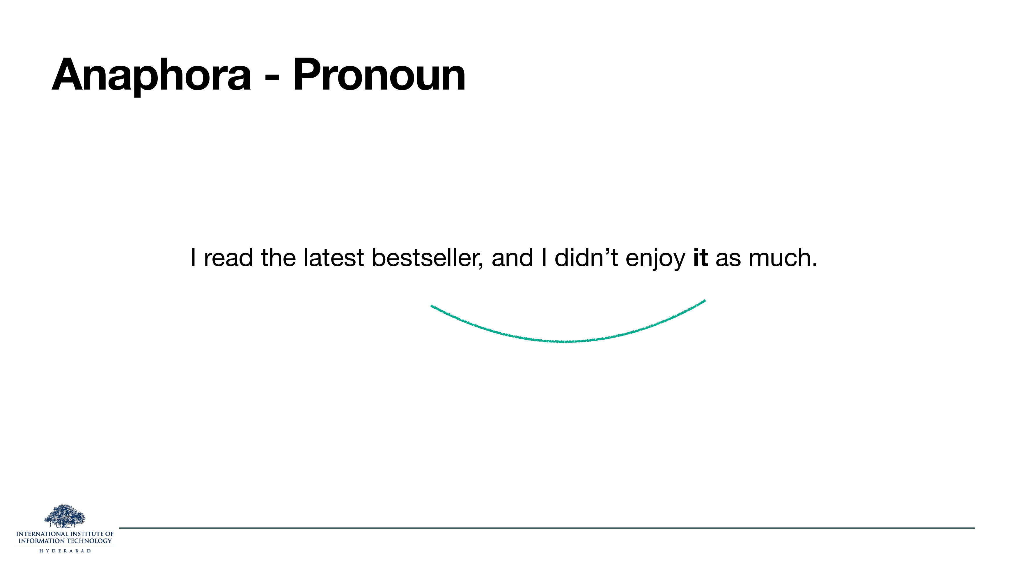
Anaphora: a pronoun refers back to something already said.
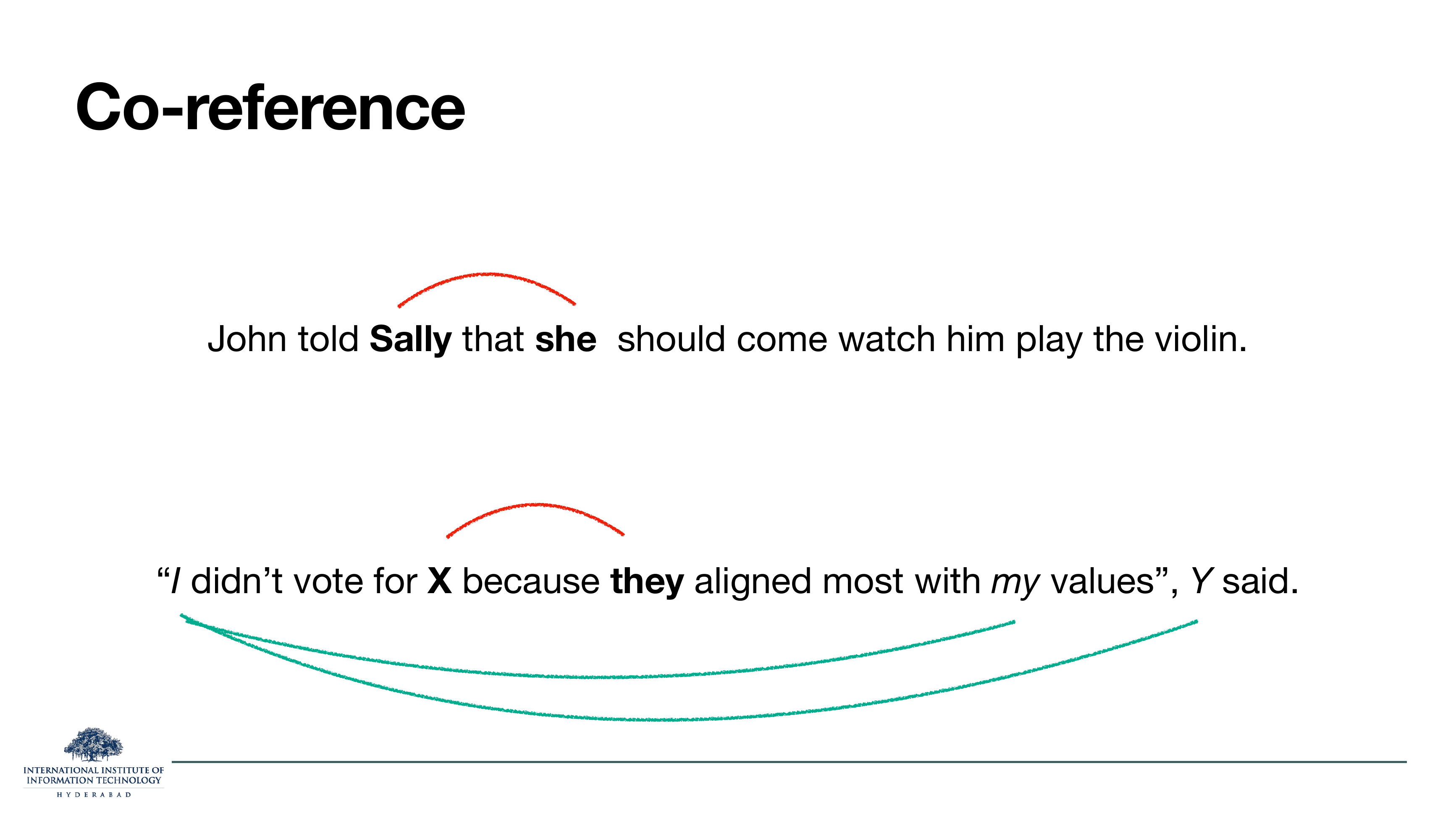
Co-reference: two mentions in a text refer to the same entity.
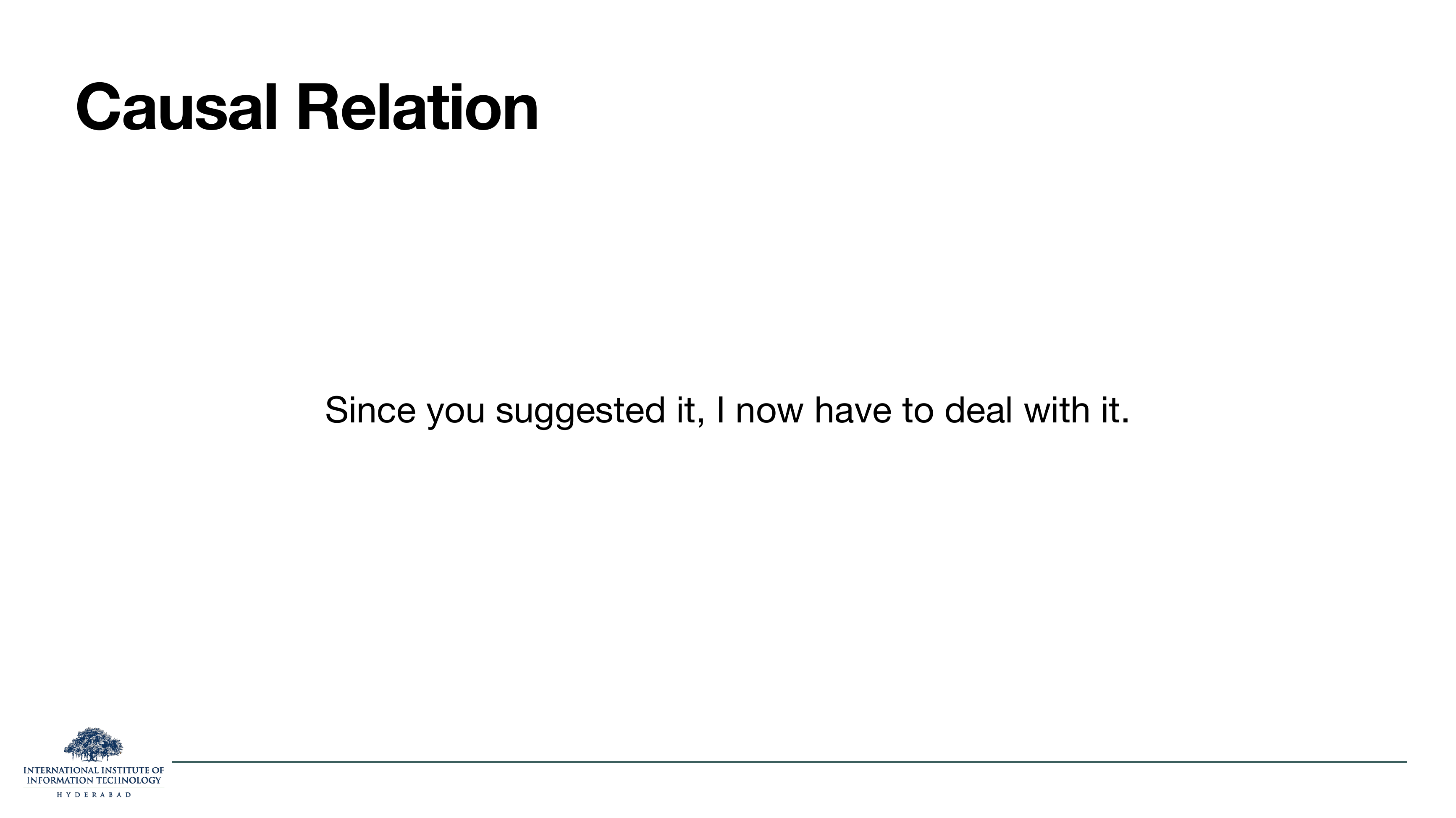
Causal: one event caused another.
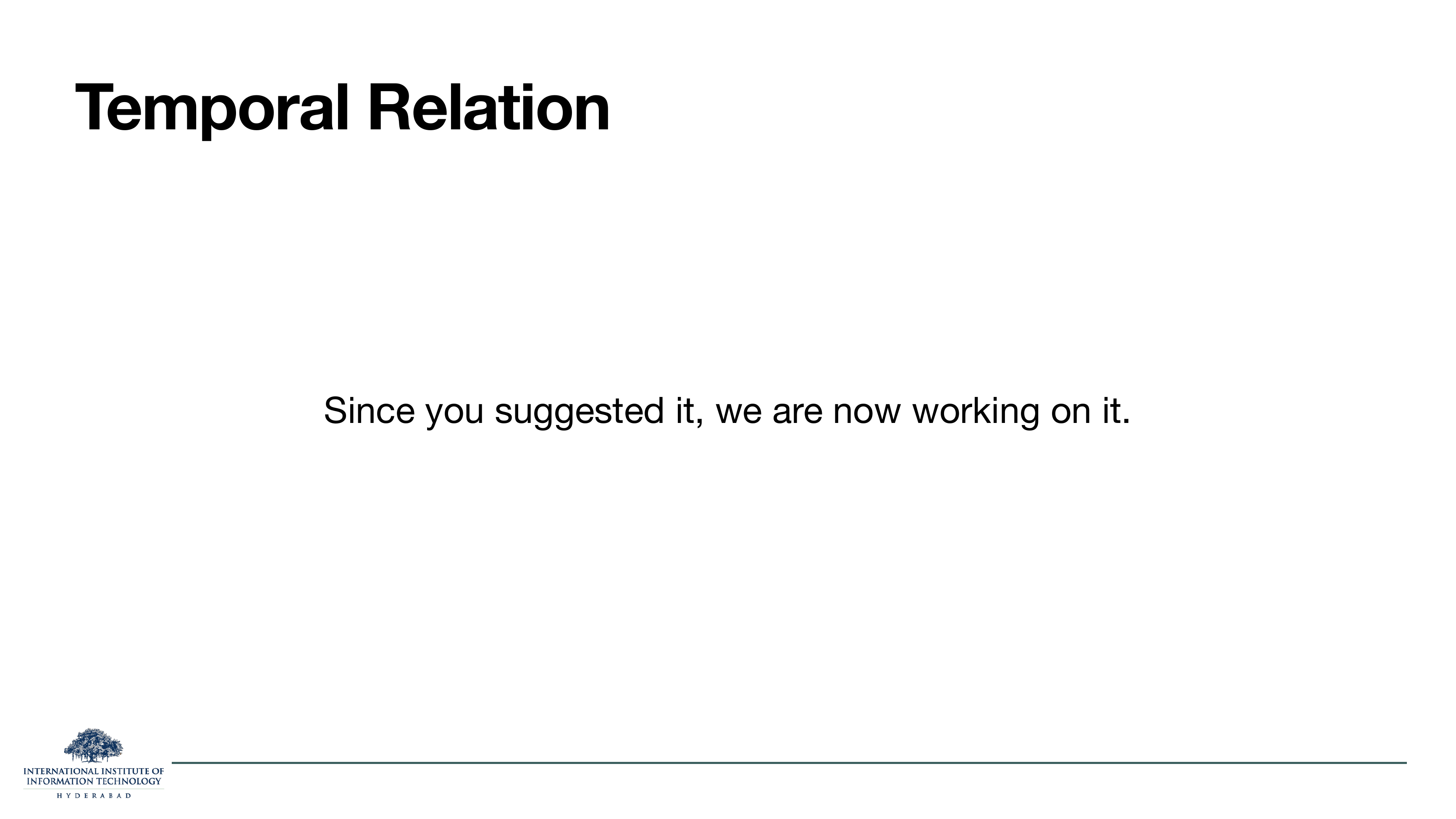
Temporal: one event happens because of, or after, another.
Discourse structures: larger organisational patterns (topic, contrast, elaboration).

The next four slides give one worked example of each of the first four.

Slide 29 / 90

Anaphora - Pronoun: 'I read the latest bestseller, and I didn't enjoy it as much.' A green arc points from 'it' back to 'the latest bestseller'.

slide 29 · anaphora

Slide 30 / 90

Co-reference: 'John told Sally that she should come watch him play the violin' with red arcs from she to Sally; and '“I didn't vote for X because they aligned most with my values”, Y said.' with arcs from I / my back to Y.

slide 30 · co-reference

On these slides

Anaphora: the pronoun "it" points back at "the latest bestseller". Co-reference: the pronoun "she" refers to "Sally"; and in the more tangled second sentence, the "I" and "my" inside the quote both refer back to "Y" outside it.

⚠ Watch out

The second example on slide 30 is a warning shot: the referent can sit outside the quoted span, and any model that scans linearly (an RNN) will find that hard. It is easy for self-attention, which can jump directly to "Y" from inside the quote. Hold that in mind when we meet attention in §6.

Slide 31 / 90

Causal relation: 'Since you suggested it, I now have to deal with it.'

slide 31 · causal

Slide 32 / 90

Temporal relation: 'Since you suggested it, we are now working on it.'

slide 32 · temporal

On these slides

The same conjunction "since" doing two completely different jobs: on slide 31 it introduces a cause ("because you suggested it…"); on slide 32 it introduces a time ("from the moment you suggested it…").

✦ Key takeaway

Same surface form, different meaning. The only way to tell them apart is to read the whole clause after "since" and pattern-match against causal versus temporal cues. A model that can only summarise the past into one fixed vector will miss the distinction; a model that can reach back and attend to the specific words that follow can catch it.

Slide 33 / 90

Long distance relation: 'When she tried to print her tickets, she found that the printer was out of ink. She went to a stationary store and purchased some ink. She felt that the ink was very expensive. After refilling the cartridge, she could finally print her ___.'

slide 33 · long-distance blank

Slide 34 / 90

Long distance relation: 'I grew up in Spain and then moved to the UK for my undergrad. After completing my undergrad I took a gap year and left for South America. I was hiking in the Patagonia and then went to Peru. While there I had no trouble speaking with the locals since I am fluent in ___.'

slide 34 · long-distance blank II

On these slides

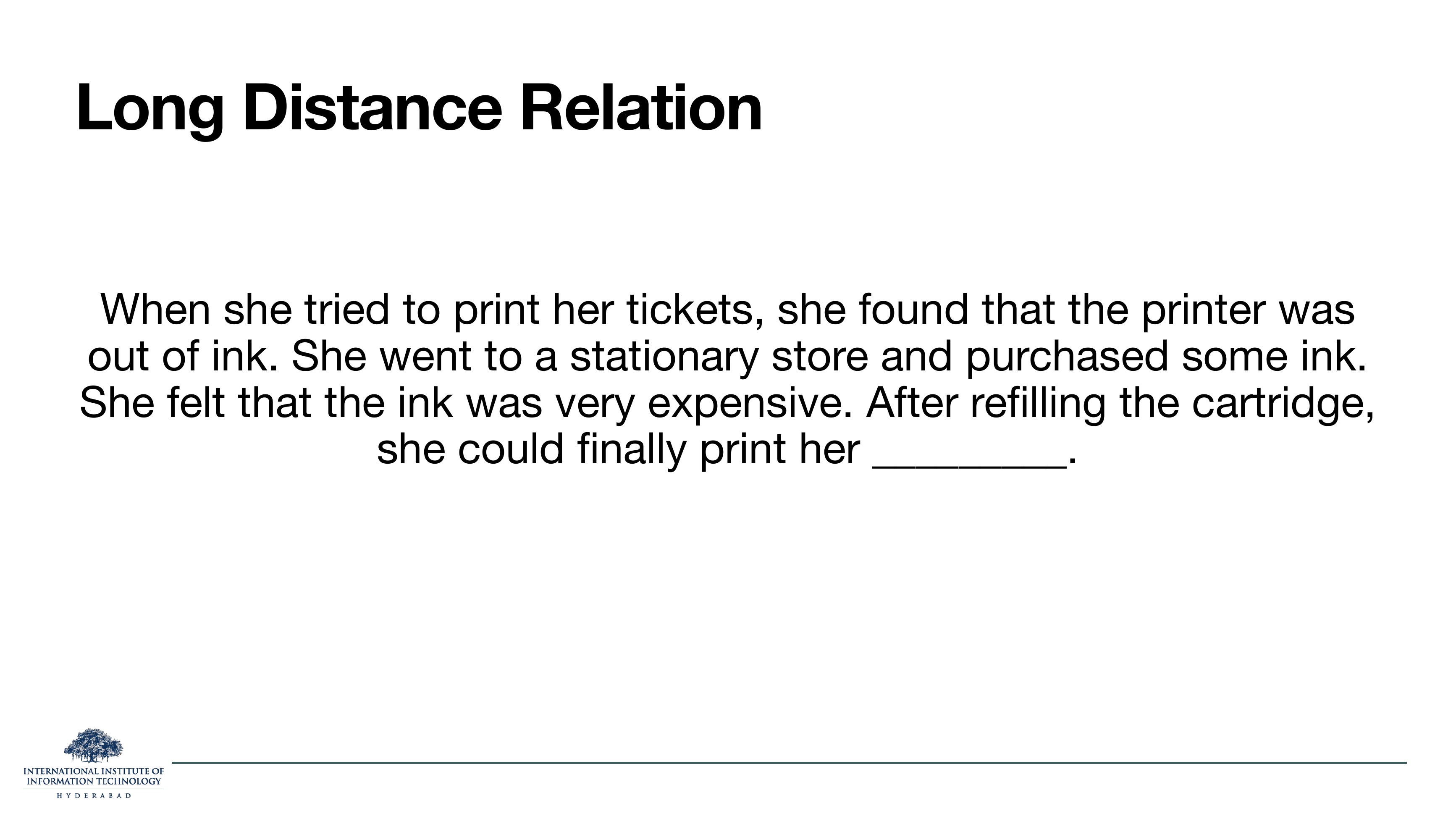
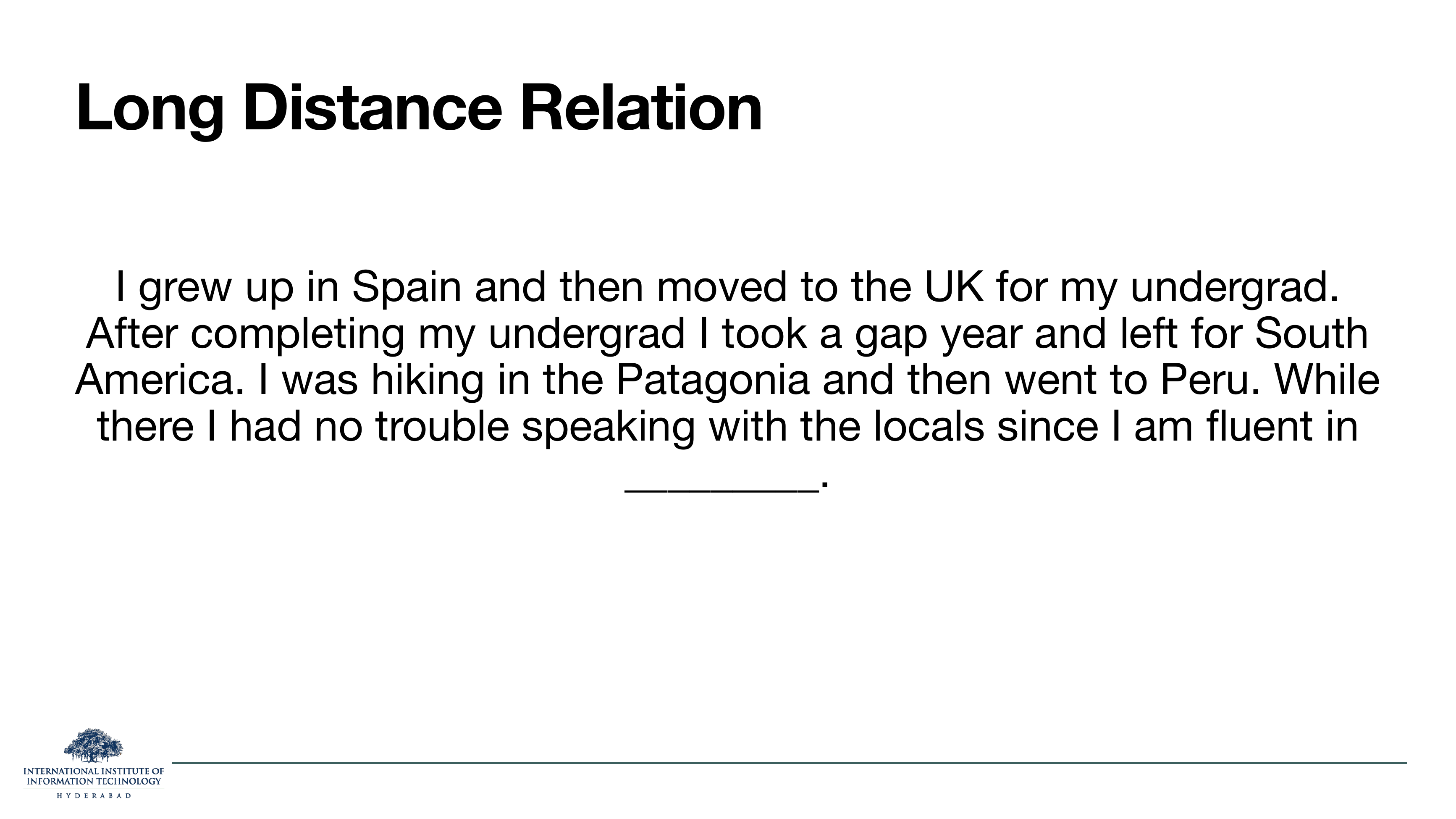
Two fill-in-the-blank paragraphs where the answer sits far back in the text.

Slide 33: the missing word is tickets, introduced in the very first clause, and never repeated. Every sentence in between is about ink.
Slide 34: the missing word is Spanish, you need to remember "grew up in Spain" from the first sentence, even though the paragraph then wanders through the UK, Patagonia and Peru.

Both examples are trivial for a fluent reader. Both are hard for an RNN whose gradient signal from that opening clause has already vanished by the end.

Slide 35 / 90

LSTM diagram (from colah.github.io): a cell with c_t-1 and h_t-1 inputs, forget gate f_t, input gate i_t, candidate c̃_t via tanh, output gate o_t; produces c_t and h_t.

slide 35 · LSTM cell

Slide 36 / 90

LSTM Advantages over RNN: vanishing gradients solved; long distance dependency partially solved (not solved for very long distances).

slide 36 · LSTM verdict

On these slides

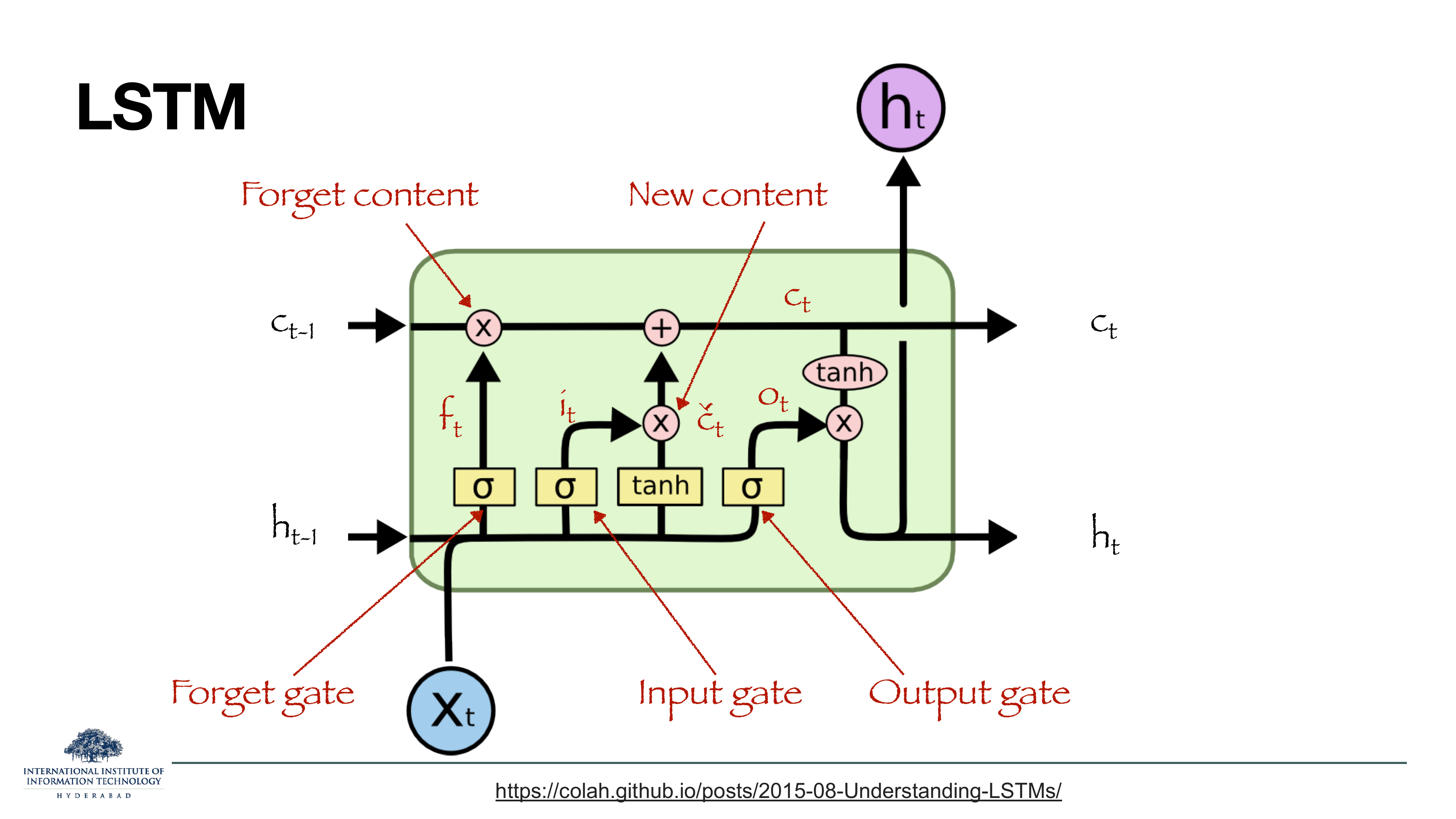
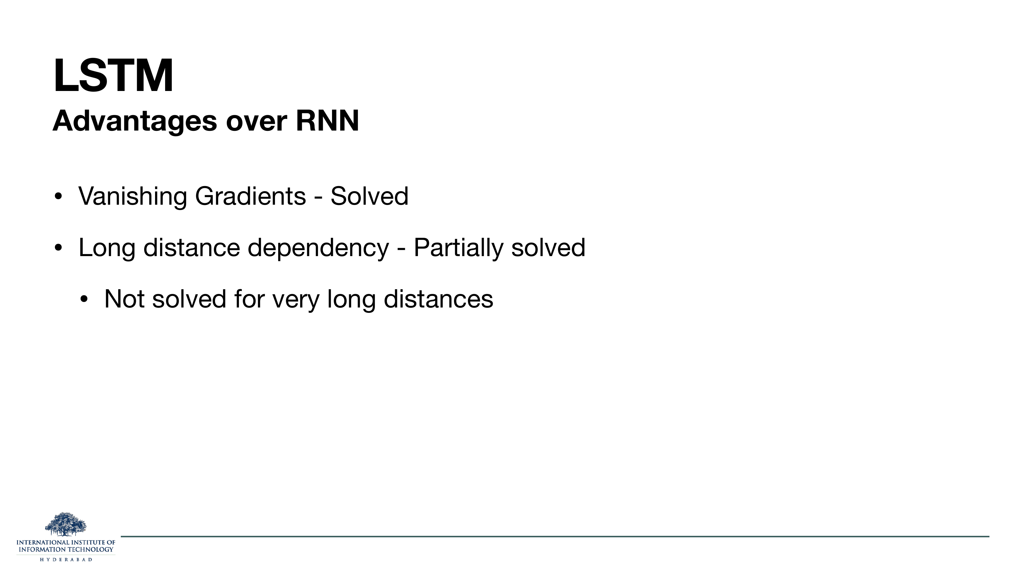
The famous Chris Olah LSTM diagram, and the honest scorecard. The LSTM adds a cell state c_t that flows through the sequence almost untouched, plus three sigmoid gates: a forget gate that decides how much of the old cell state to keep, an input gate that decides how much of the newly-computed candidate to add, and an output gate that decides how much of the cell state to expose as the hidden state.

Under the hood

Why does this fix vanishing gradients? Because the cell state is passed forward via addition, not repeated multiplication. Additive updates give the gradient a straight path back to the beginning of the sequence. No more exponential decay.

Why it isn't the end of the story

Slide 36 is honest: LSTMs partially solve long-distance dependency. They still process one token at a time, so the parallelism problem remains, and for really long documents (a hundred sentences apart) their memory still degrades. This is the door the transformer walks through.

§6Attention as the fix

Nine slides. First the lecture closes the LSTM chapter with its residual limitations, then it walks Bahdanau attention (2015) through a three-word machine-translation example, one output token at a time. This is the moment the deck turns: the same attention gadget you see wrapped around an RNN here becomes the entire model in the next section.

Slide 37 / 90

LSTM Limitations: computationally complex, slow, limited long-distance dependency, transfer learning not possible.

slide 37 · LSTM's residual sins

On the slide

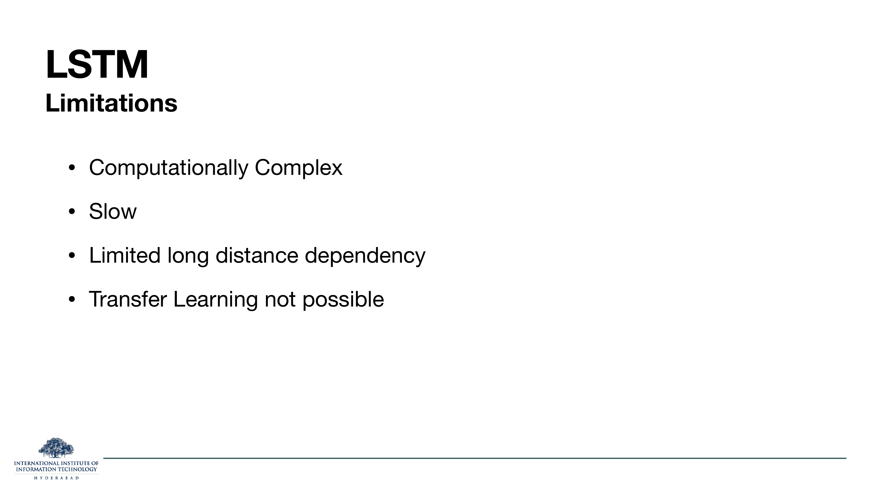
Four remaining problems the LSTM cannot fix. It is computationally complex (four gates means four matrix multiplies per token), it is slow (still sequential in time), long dependencies degrade past a few dozen tokens, and there is no clean recipe for transfer learning: you cannot easily pretrain a giant LSTM on the web and then fine-tune it on your task.

→ Keep reading

The transfer-learning point is what BERT and GPT eventually solved, and they could only do it because the architecture underneath (the transformer) is parallelisable at pretraining scale.

Slide 38 / 90

slide 38 · section divider

Section divider. Everything from here is about attention, from its Bahdanau-2015 origins to full self-attention.

Slide 39 / 90

Seq2Seq encoder–decoder for machine translation: encoder reads 'I like coffee' one token at a time, producing a single 'encoder vector'; decoder consumes that vector and emits 'Me gusta ...' one token at a time.

slide 39 · plain seq2seq

Slide 40 / 90

Encoder–decoder limitation: the same picture, but the vertical 'encoder vector' at the boundary is annotated as 'Information Bottleneck'.

slide 40 · the bottleneck

On these slides

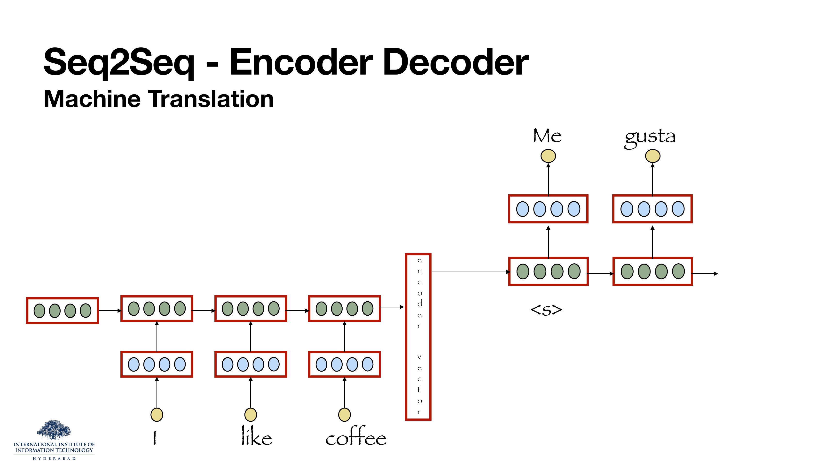
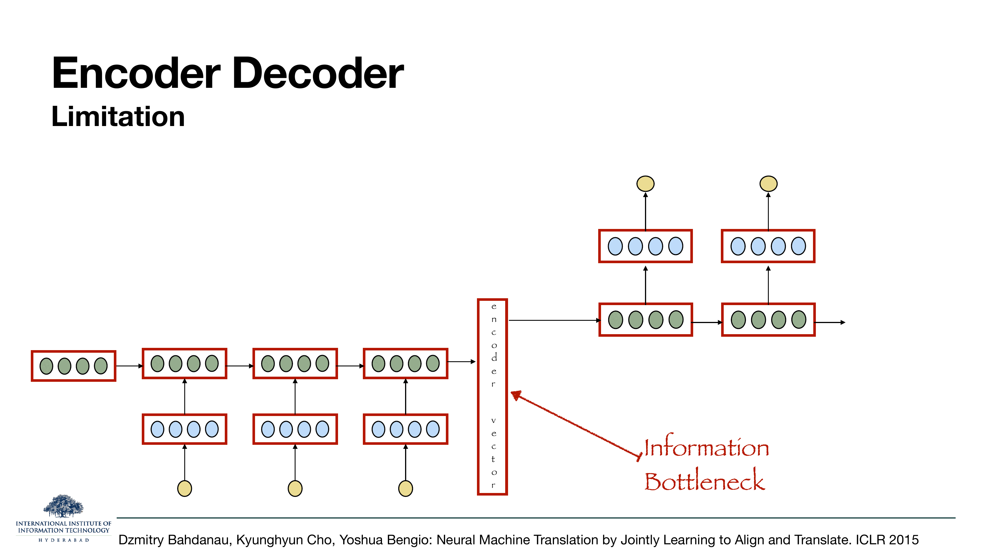
The pre-attention seq2seq model for machine translation (Sutskever, Vinyals & Le, 2014): an encoder RNN reads the source sentence "I like coffee" and squeezes it into a single fixed-size encoder vector; a decoder RNN then generates the target "Me gusta el café" from that vector.

⚠ the bottleneck

Every last drop of information about the source has to fit into that one vector. A 20-word sentence, a 200-word sentence, a whole paragraph, all the same size. This is the "information bottleneck" the arrow on slide 40 is pointing at, and it is exactly what Bahdanau, Cho and Bengio (ICLR 2015) proposed to fix.

Slide 41 / 90

Attention: more information from the sentence before translating; each decoder step uses a direct connection to the encoder. A bar chart shows a peaked distribution over input words when producing 'Me gusta el café' from 'I love coffee'.

slide 41 · what attention buys

On the slide

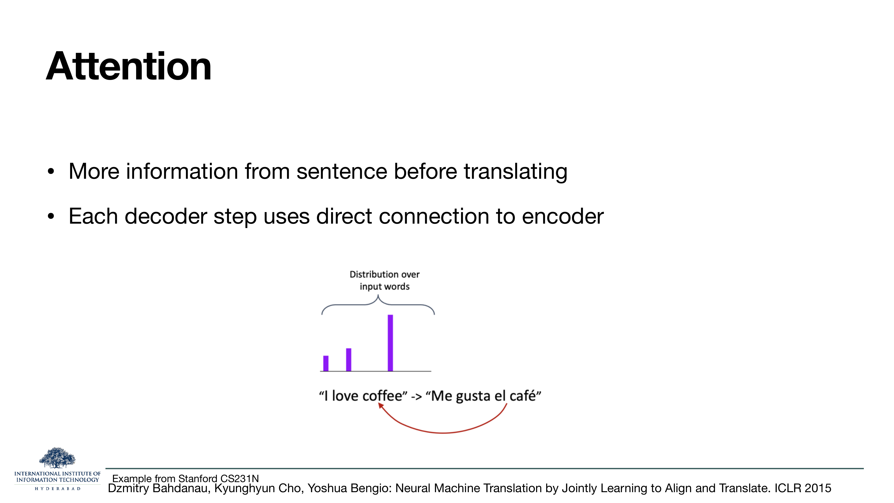
The pitch. At every decoder step, instead of relying only on the summary vector, the decoder looks back at all the encoder hidden states and takes a weighted combination of them, with the weights (the attention distribution) computed on the fly.

What it means

The decoder gets to choose, at each output word, which source words to focus on. Producing "café" attends heavily to "coffee"; producing "Me" attends to "I". No single vector has to remember the whole sentence, because the whole sentence is still there for the decoder to look at.

Slide 42 / 90

Attention step 1: decoder is at the start token, computes attention scores against each encoder state, produces a distribution peaked on 'I', gets an attention output which combined with the decoder state gives 'Me'.

slide 42 · producing "Me"

Slide 43 / 90

Attention step 2: decoder consumes 'Me', now attention distribution peaks on 'like', producing 'gusta'.

slide 43 · producing "gusta"

Slide 44 / 90

Attention step 3+: the finished translation 'Me gusta el café' produced token by token; attention peaks on 'coffee' when producing 'café'.

slide 44 · producing "café"

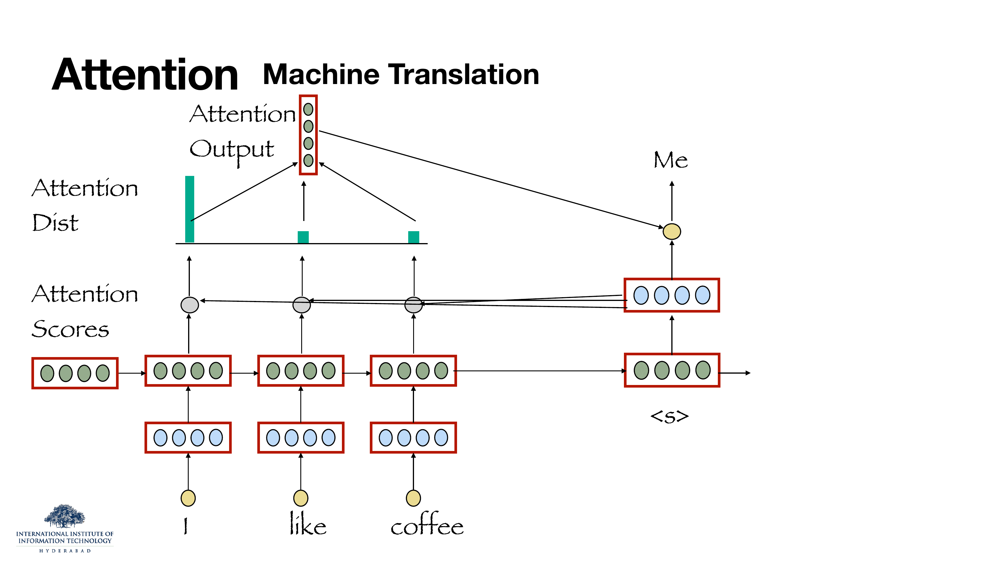
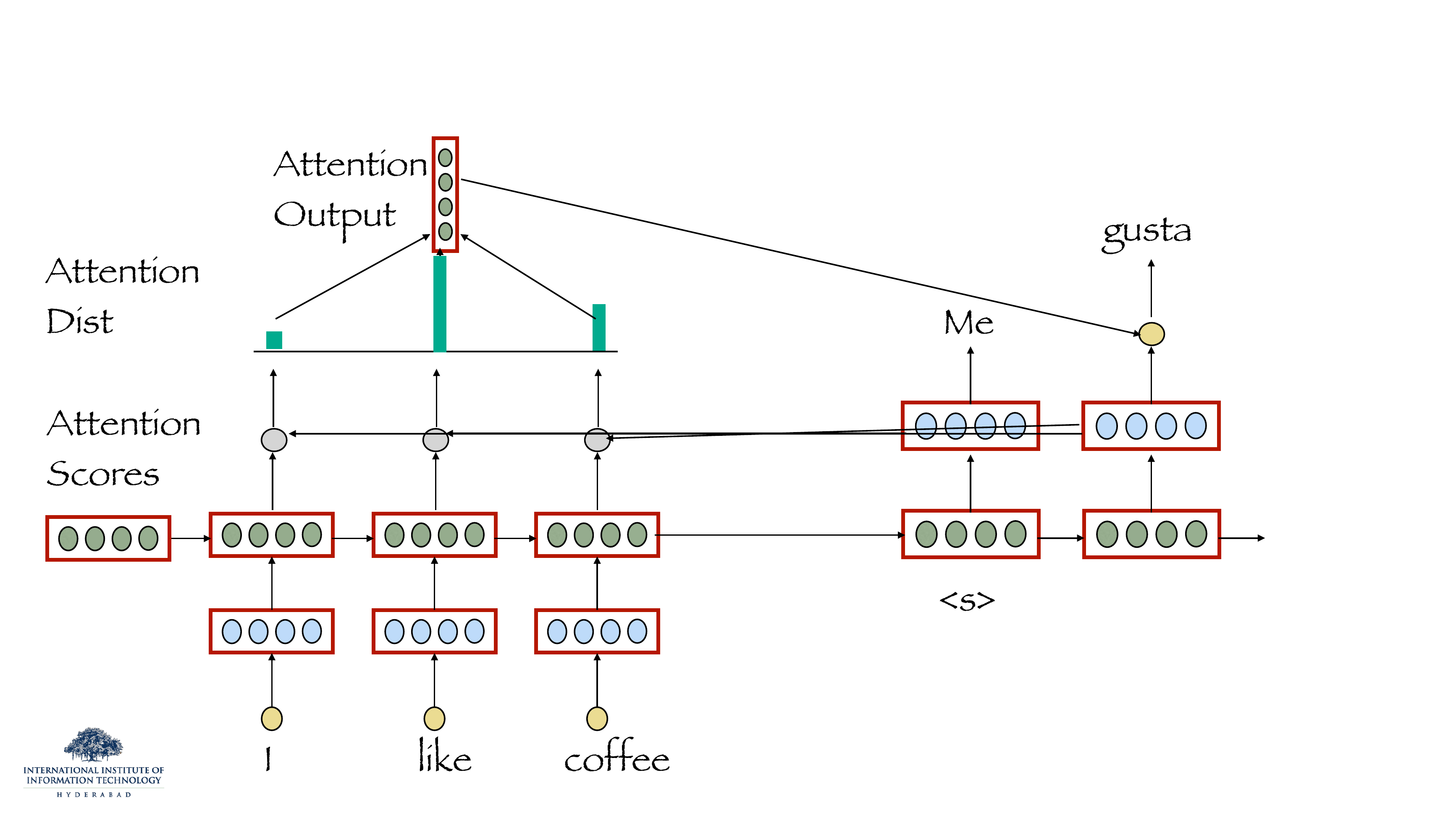
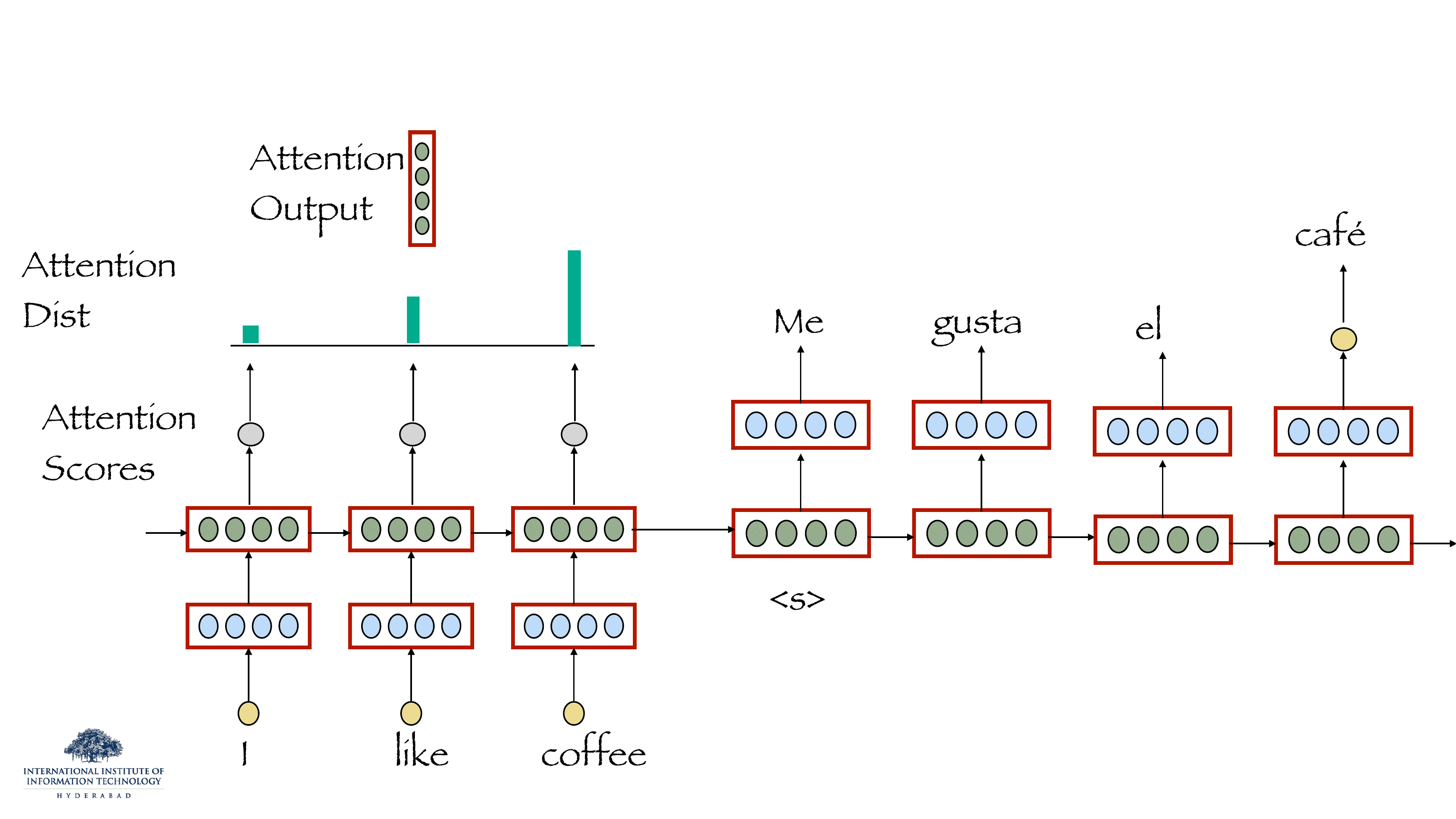
On these slides

Three snapshots of the same decoding, at different output positions. At each step:

The decoder state is compared against every encoder state to produce attention scores.
Those scores are softmaxed into an attention distribution.
The distribution is used to weight-sum the encoder states, producing an attention output.
The attention output is concatenated with the decoder state and used to predict the next word.

Under the hood

The attention distribution changes at every output token; that is why we see three different peaked bar charts in three consecutive slides. Same encoder, same decoder, different soft look-ups.

✦ Key takeaway

Watch what the attention distribution is doing on slide 44. It peaks on "coffee" when producing "café". Nobody told it to. It learned it from data. This is where the "attention as soft alignment" intuition comes from, and why classical machine-translation alignment tables became obsolete overnight.

Slide 45 / 90

Attention Advantages: no information bottleneck (no one hidden state to capture all source info); each decoder step uses direct connection to encoder; more 'human-like' process; attention distribution gives some interpretability; no explicit alignment needed.

slide 45 · attention scorecard

On the slide

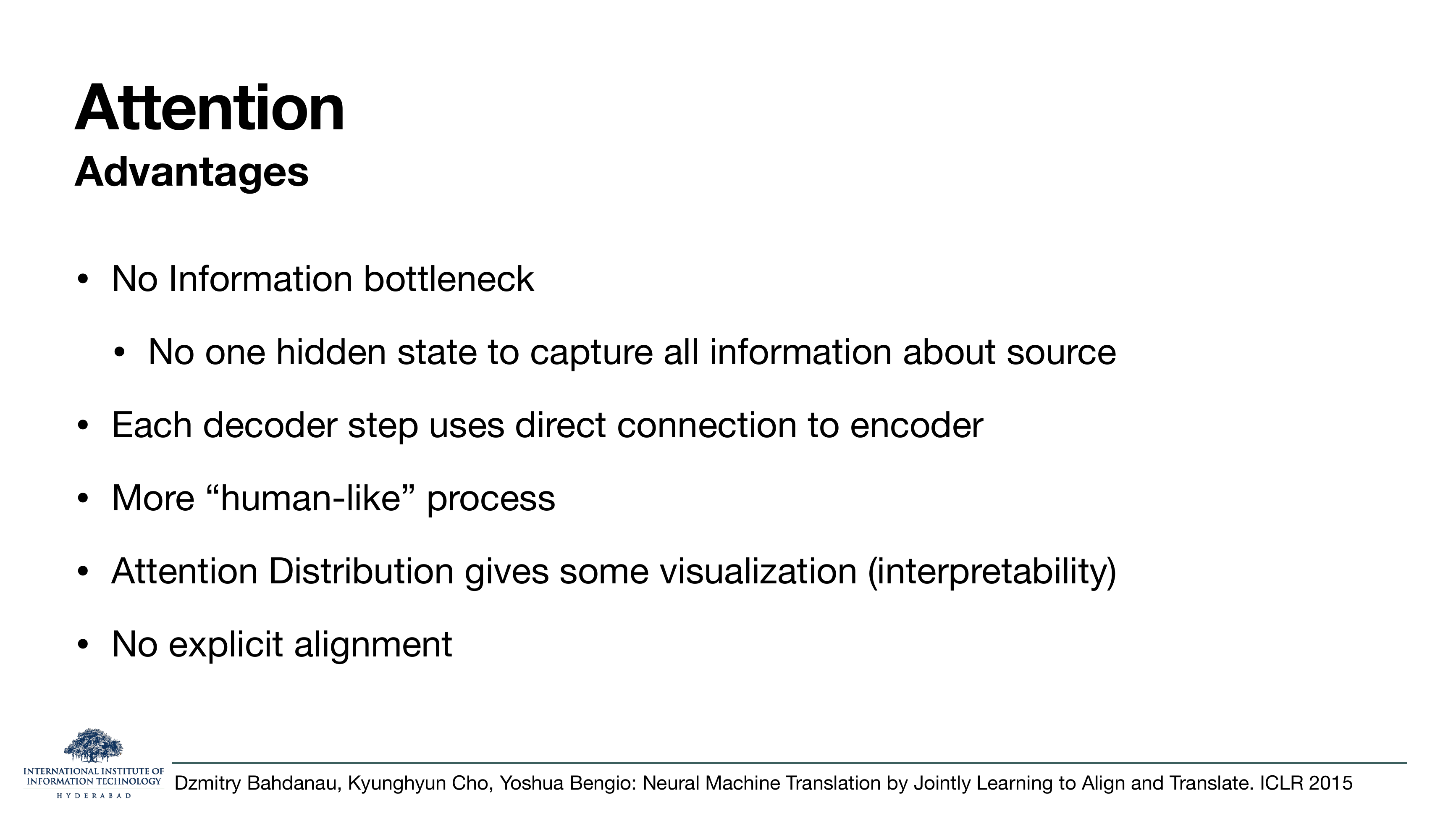
Five wins over plain seq2seq. The first two are the mechanical fix (no bottleneck, direct source access). The third is the intuition ("humans do not read a whole sentence into a single vector before translating either"). The fourth is a big deal in practice, attention weights can be plotted as a heatmap and give you a rough visualisation of what the model is looking at. The fifth is the surprise: statistical machine translation before this had a whole subfield on learning explicit word alignments; attention gets alignment for free as a byproduct.

§7Self-attention and multi-head

Twenty slides. The lecture takes the attention gadget from the last section, throws away the RNN it was wrapped around, and asks: what if we let a sequence attend to itself? What follows is the entire transformer machinery, one operation at a time, embeddings, then queries/keys/values, then the attention matrix, then multi-head, then the scorecard against RNN. By slide 65 you have the "Attention is All You Need" paper's centrepiece.

Slide 46 / 90

Attention Issues with RNN/LSTM: long distance dependency, sequential processing.

slide 46 · leftover RNN issues

On the slide

A summary of what attention could not fix when it was still bolted onto an RNN. The RNN underneath still runs sequentially and still degrades on very long dependencies. To get rid of both we need to get rid of the RNN.

Slide 47 / 90

Transformer: title page of 'Attention Is All You Need' by Vaswani et al., NeurIPS 2017.

slide 47 · the paper

On the slide

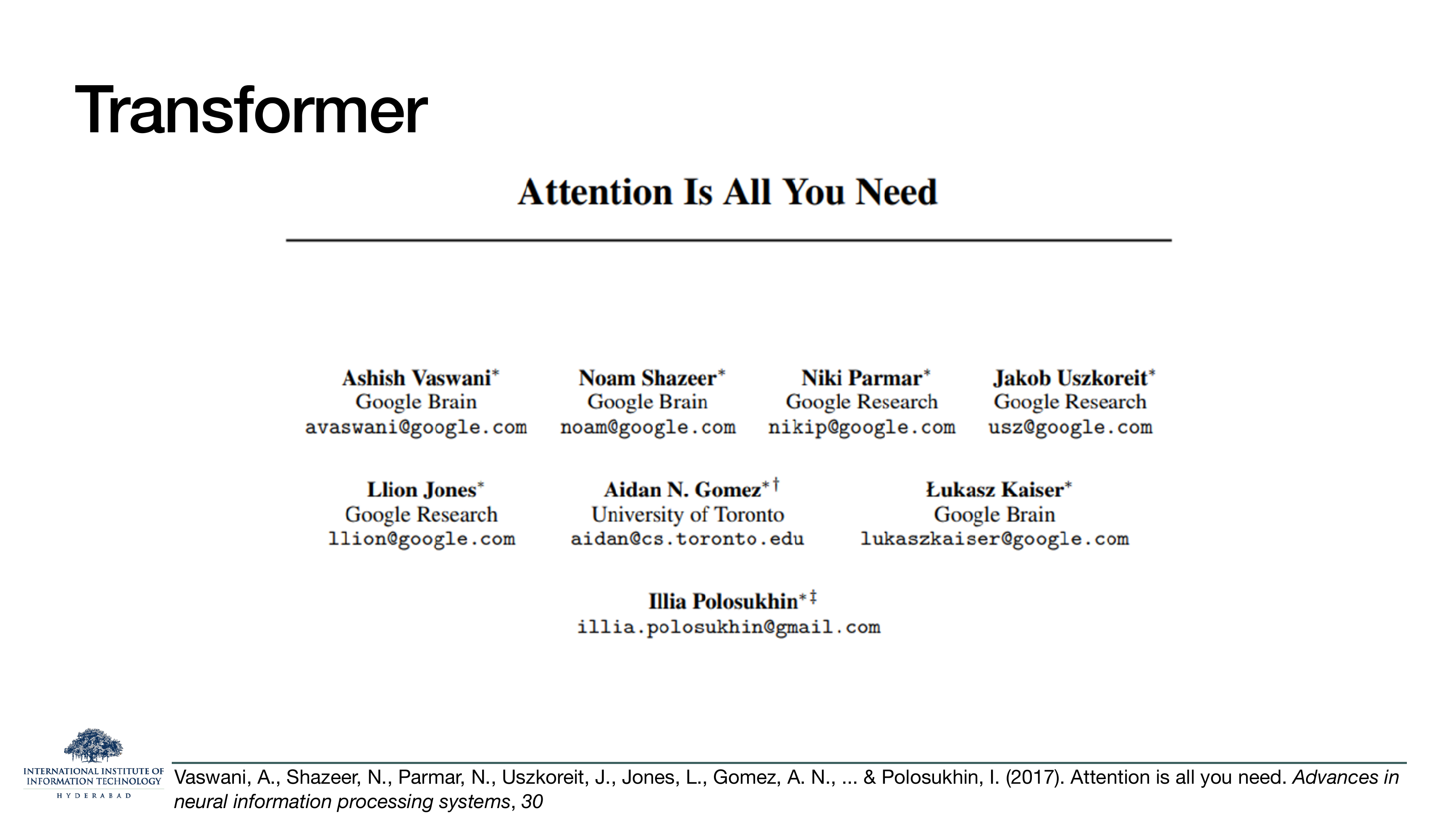
The title page of Vaswani et al., Attention Is All You Need (NeurIPS 2017). Eight authors, all at Google.

✦ Key takeaway

Read the title as a claim. It says: given attention, you do not need a recurrence at all. Every part of the RNN that attention was patching over, the encoder, the decoder, the recurrence in between, can be replaced by more attention. The rest of the deck spells out how.

Slide 48 / 90

slide 48 · section divider

Sub-divider. From here through slide 65 we build self-attention step by step.

Slide 49 / 90

Self-attention basics: 'The animal didn't cross the street because it was too tired'. Every word connects to every other word with arcs.

slide 49 · everything attends to everything

Slide 50 / 90

Tensor2Tensor attention visualization at layer 5: the pronoun 'it_' attends strongly to 'The_ animal_' — self-attention has resolved the anaphora.

slide 50 · "it" finds "the animal"

On these slides

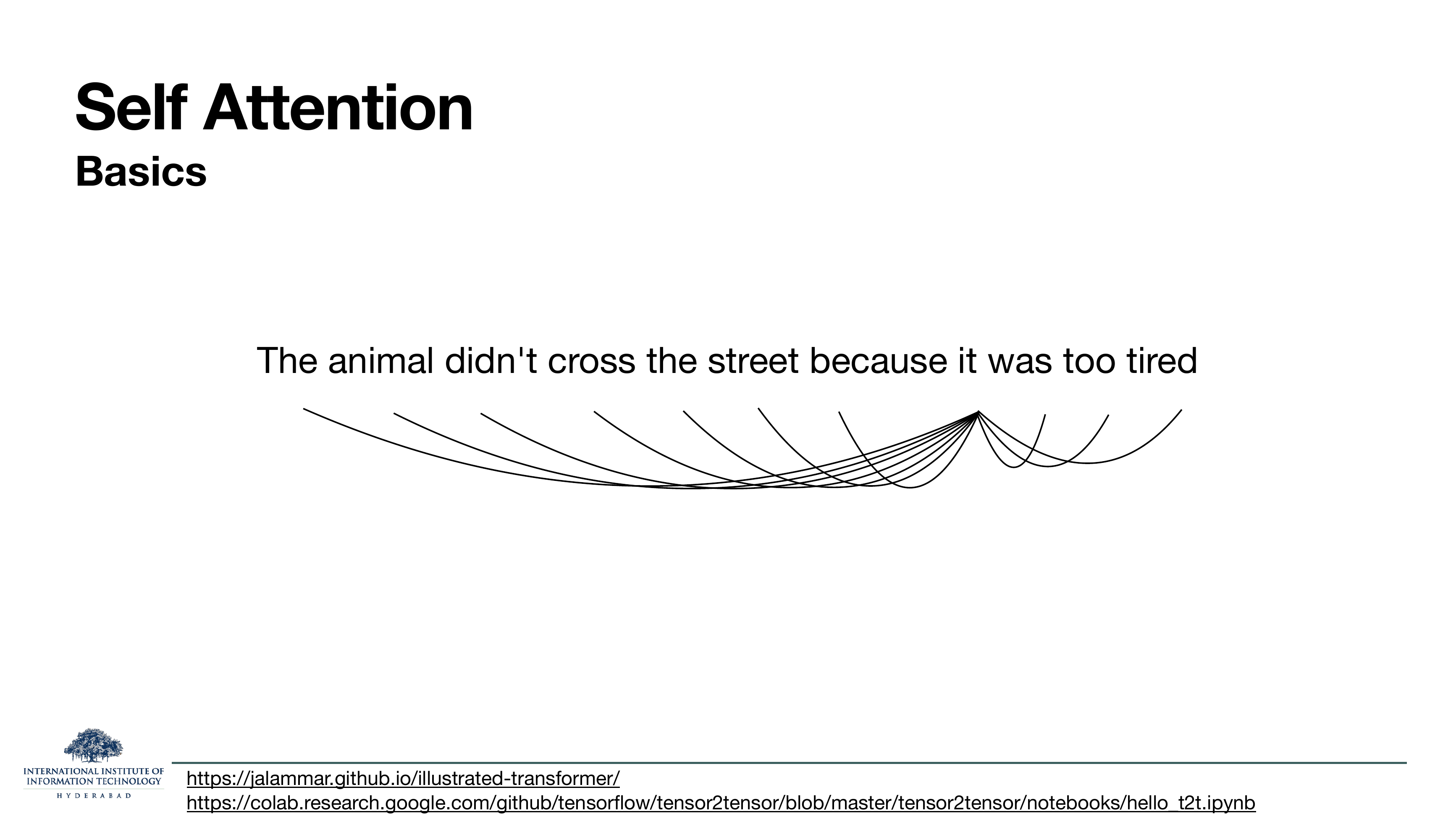
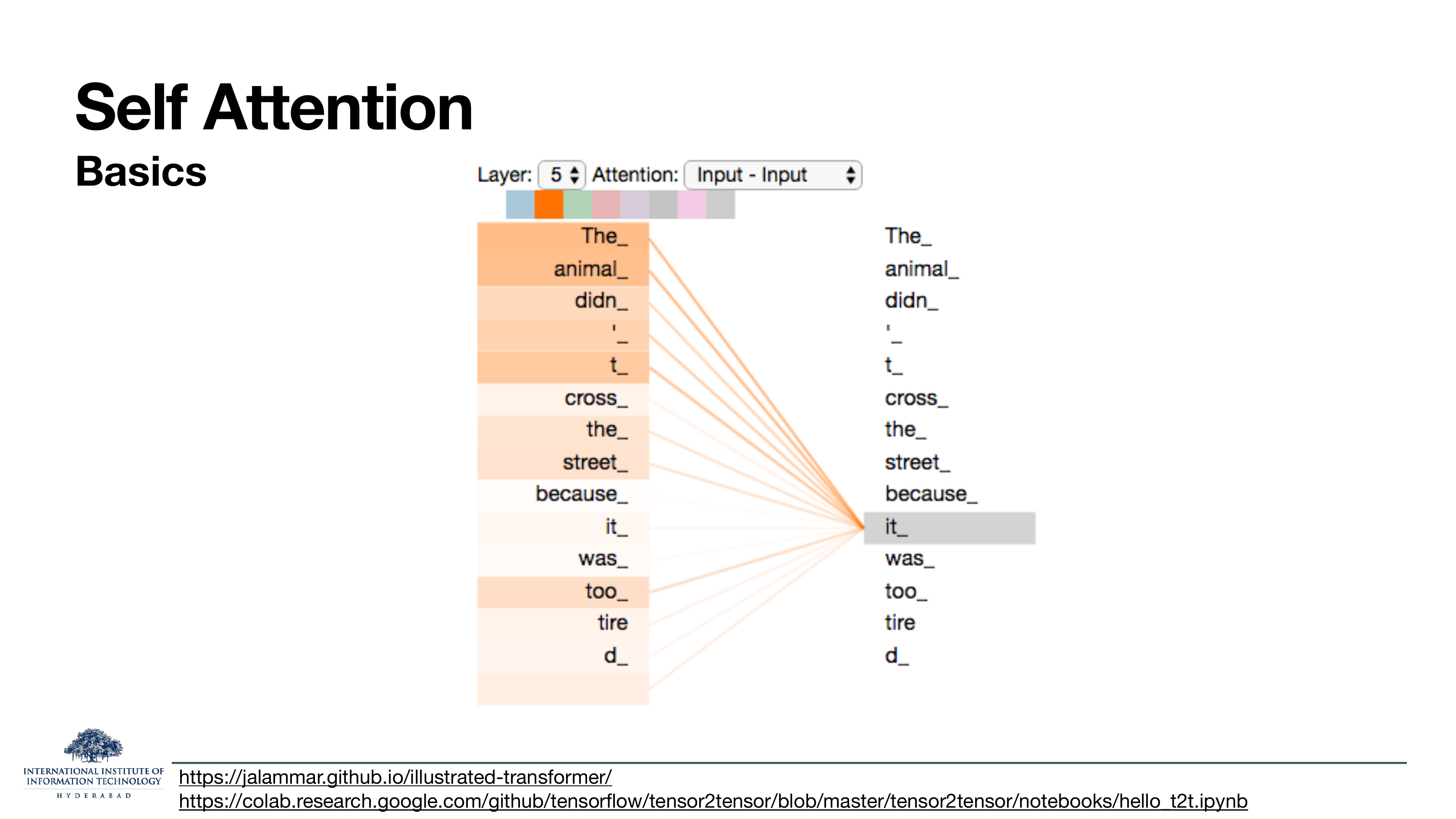
The core idea of self-attention: within a single sentence, let every position attend to every other position. Slide 49 draws the arcs; slide 50 shows what a trained transformer actually does on the sentence "The animal didn't cross the street because it was too tired". The token "it" learns to attend heavily to "the animal", the model has silently resolved an anaphora with no explicit supervision.

✦ Key takeaway

Compare this to the arcs on slide 29. What was called "anaphora" back there and demanded a special linguistic algorithm is here just what one of the attention heads at layer 5 does for free.

Slide 51 / 90

Self-attention embedding: two copies of 'The cute fluffy brown cat is lazing over the bright shelf in the corner'. Arcs from 'cat' pull in cute/fluffy/brown; arcs from 'shelf' pull in bright and 'corner'.

slide 51 · context-aware embeddings

On the slide

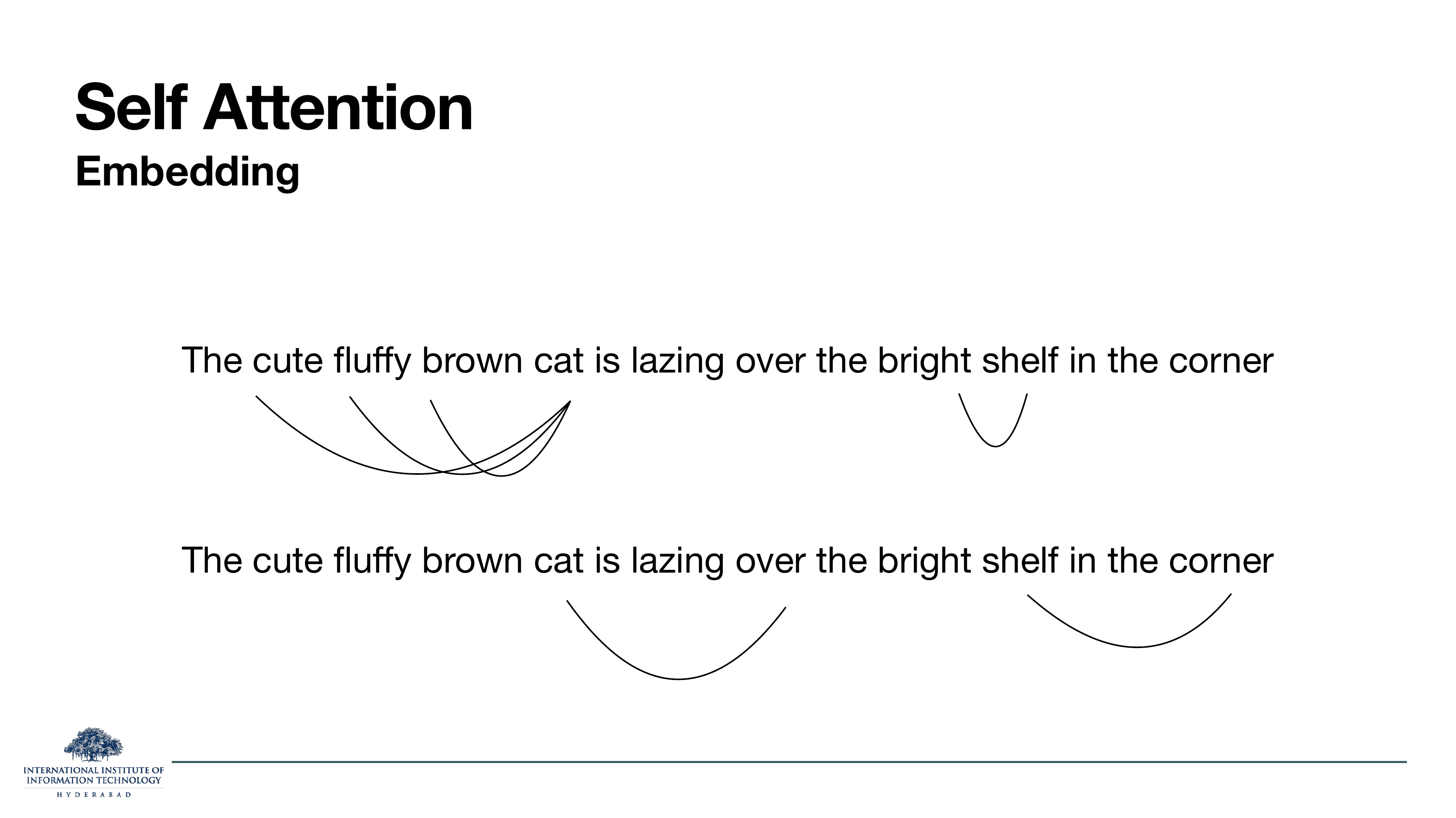
The intuitive job description for self-attention. The word "cat" starts life as a plain type-level embedding; after one self-attention layer, its representation has soaked up "cute", "fluffy" and "brown" (the adjectives that modify it). Meanwhile "shelf" absorbs "bright" and "corner".

Why this matters

This is exactly the "contextual embedding" property that Word2Vec did not have and BERT did. Self-attention is the mechanism that turns a static word embedding into a sentence-dependent one.

Slide 52 / 90

Empty attention matrix indexed by rows and columns of 'A brown cat lazes on the shelf'. Every pair of tokens gets one cell.

slide 52 · empty matrix

Slide 53 / 90

Self-Attention calculation formula: Attention(Q,K,V) = softmax(QK^T / sqrt(d_k)) V.

slide 53 · the formula

On these slides

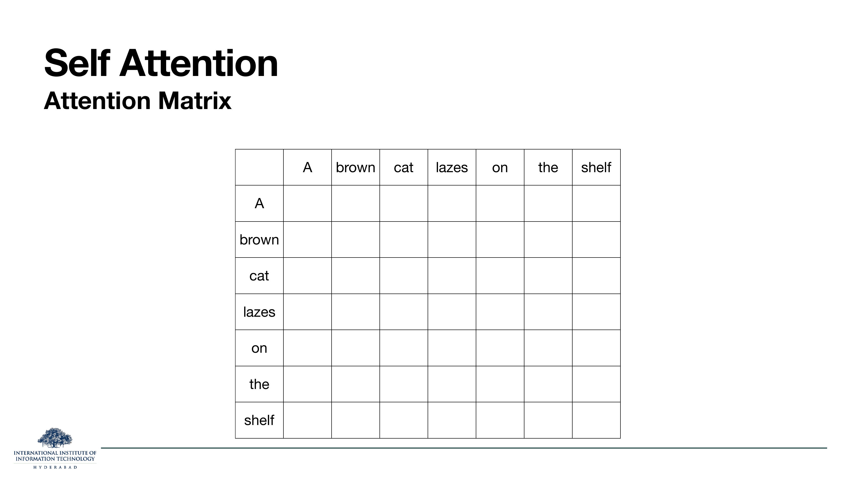
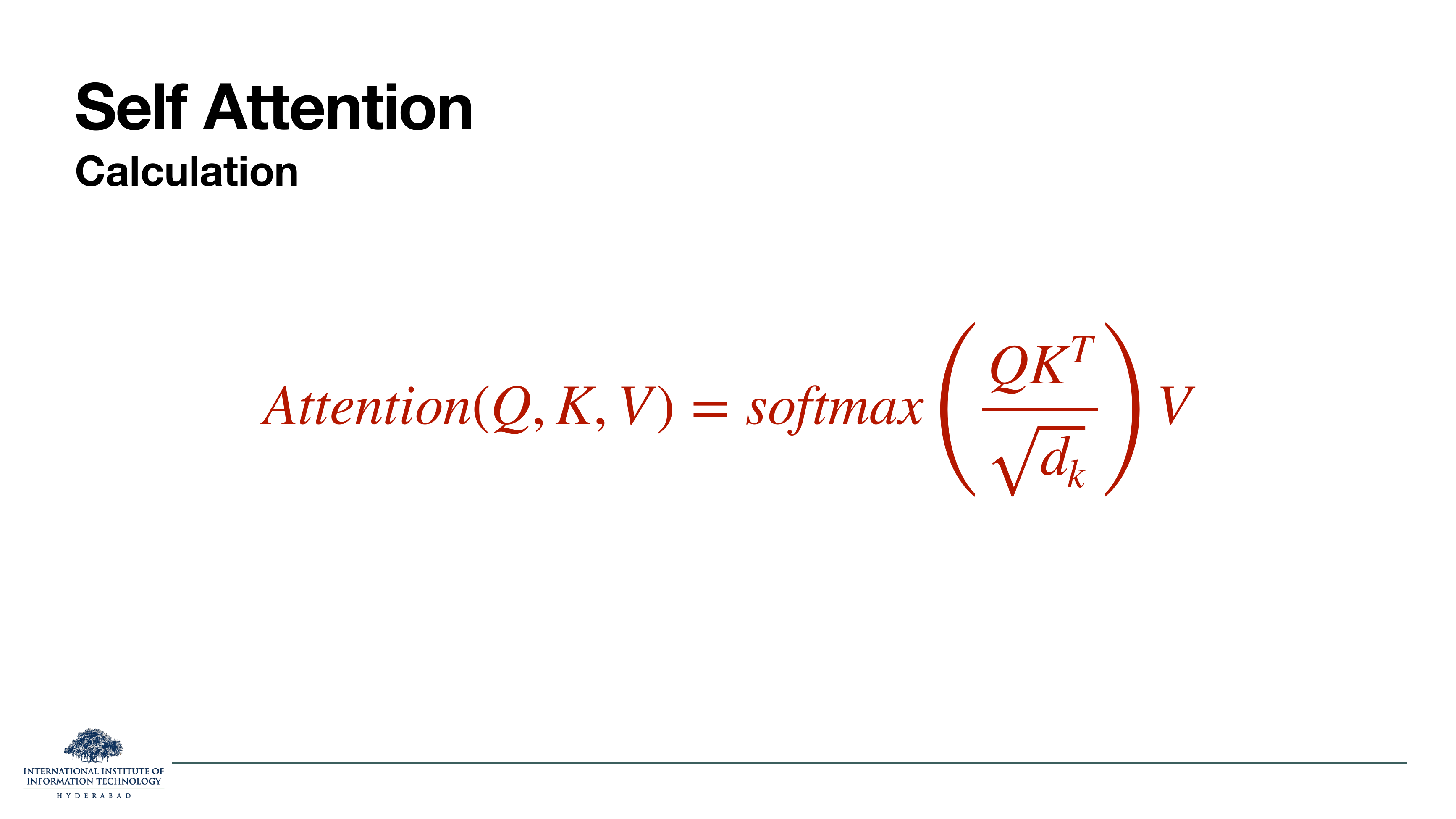
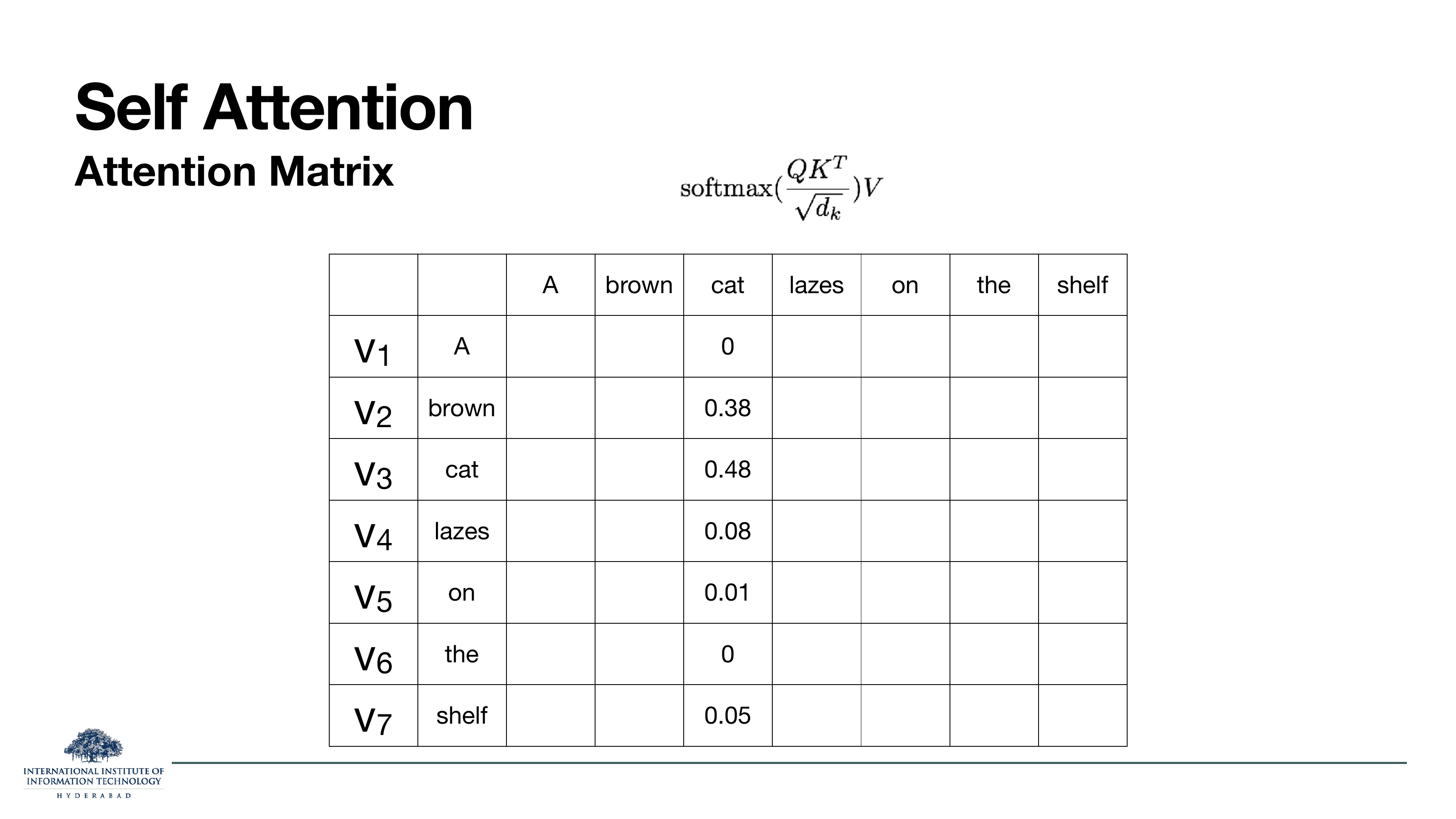
The bookkeeping. Slide 52 sets up an n×n matrix where each cell says "how much should the row-token attend to the column-token?" Slide 53 gives the one equation that fills it in:

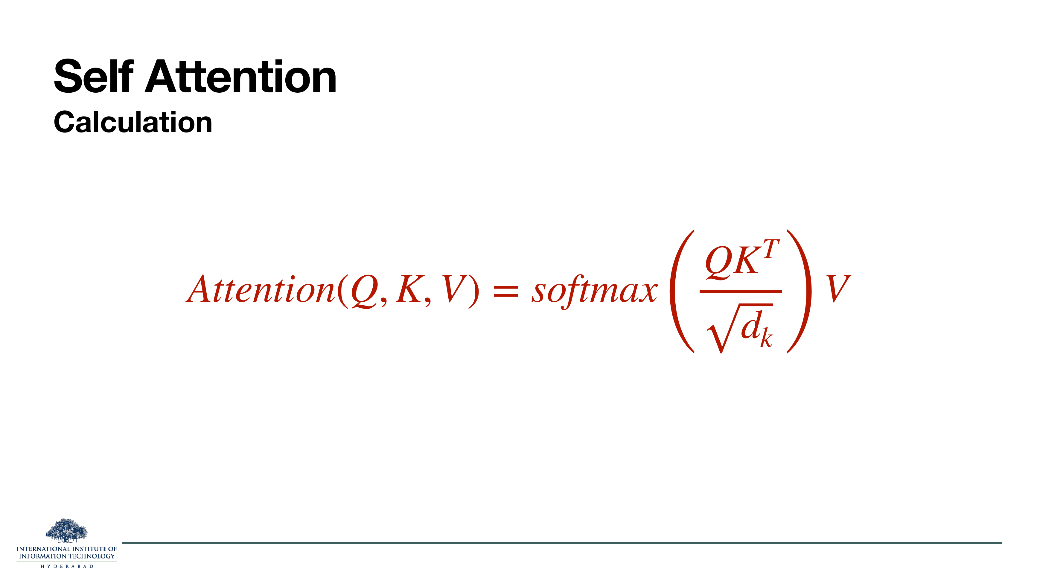
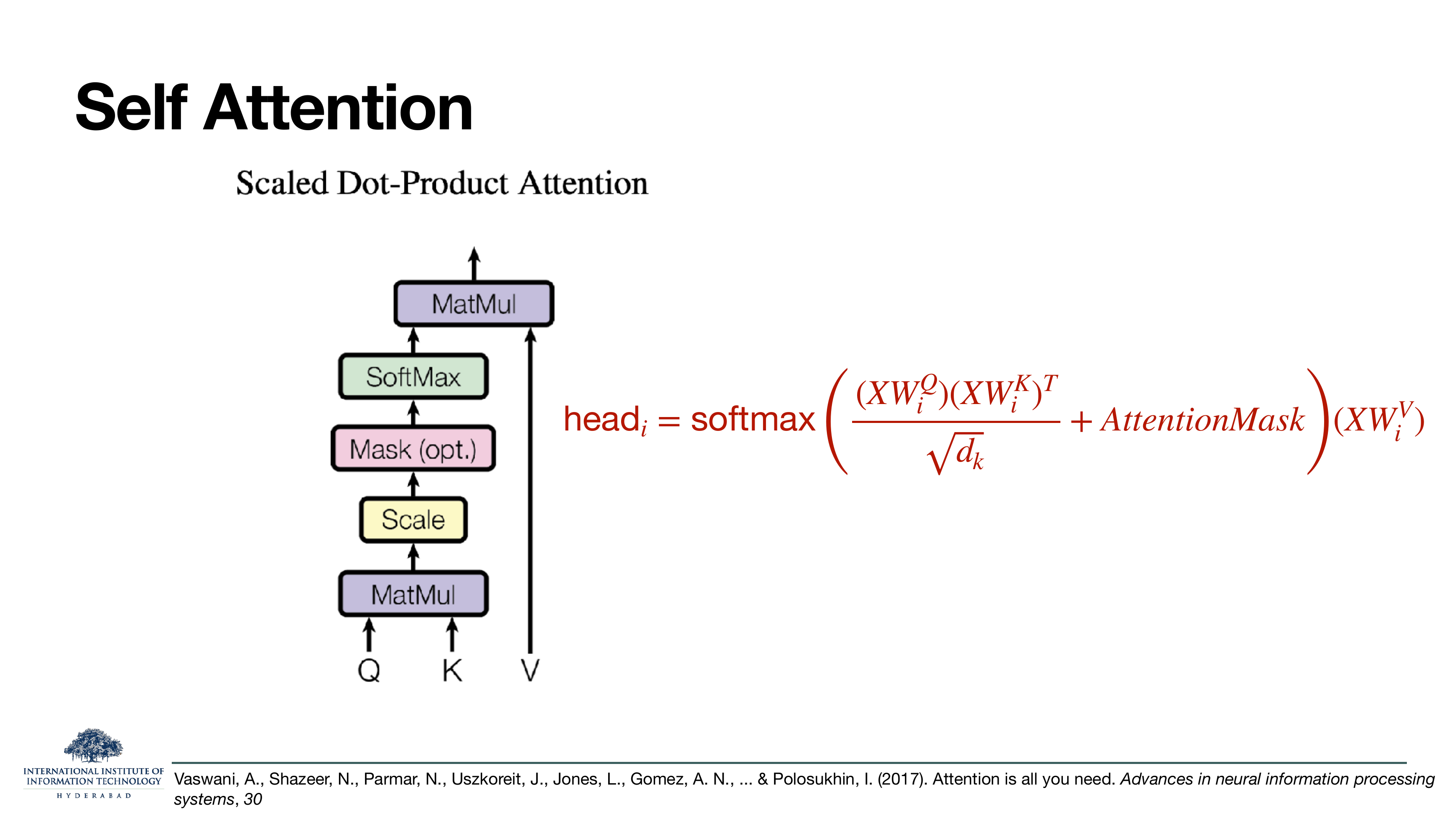
Attention (Q, K, V) = softmax (\frac{Q K^{T}}{\sqrt{d_{k}}}) V

Three inputs, queries Q, keys K, values V, and one scalar hyperparameter d_k, the key dimension. Compute pairwise dot products between queries and keys, scale down by √d_k, softmax across the row, then use those weights to average the values.

Under the hood

The scale factor √d_k is not cosmetic. Without it, large key dimensions give dot products with huge variance, which push softmax into saturated regions where its gradient is tiny. Dividing by √d_k keeps the pre-softmax scores at unit variance and gradients healthy.

Slide 54 / 90

Every token 'A brown cat lazes on the shelf' gets an embedding E_1 ... E_7.

slide 54 · embeddings

Slide 55 / 90

Each token gets three vectors k_i, q_i, v_i.

slide 55 · three vectors per token

Slide 56 / 90

Transform word embeddings with weight matrices: k = E W_K, q = E W_Q, v = E W_V.

slide 56 · where Q/K/V come from

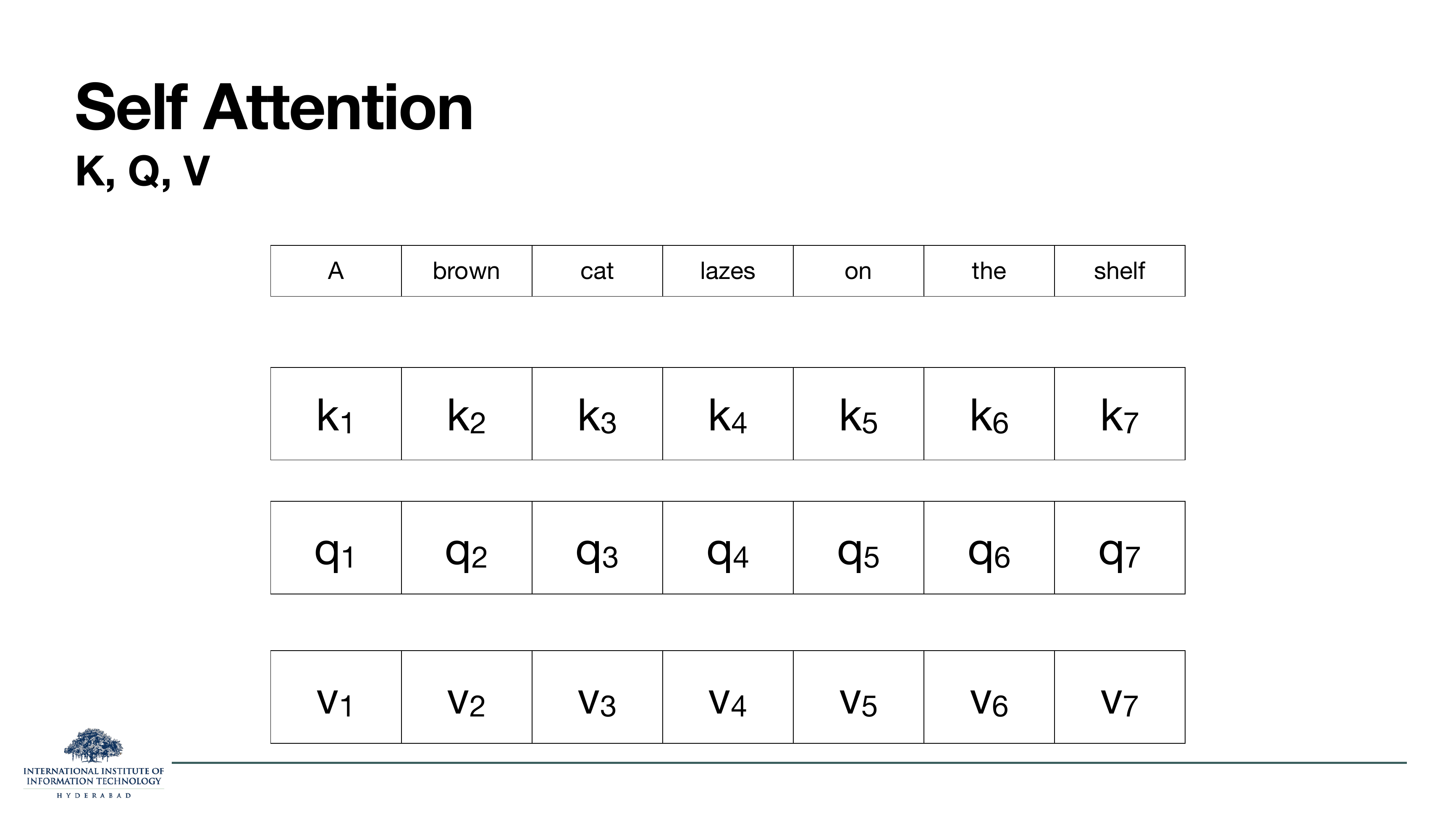
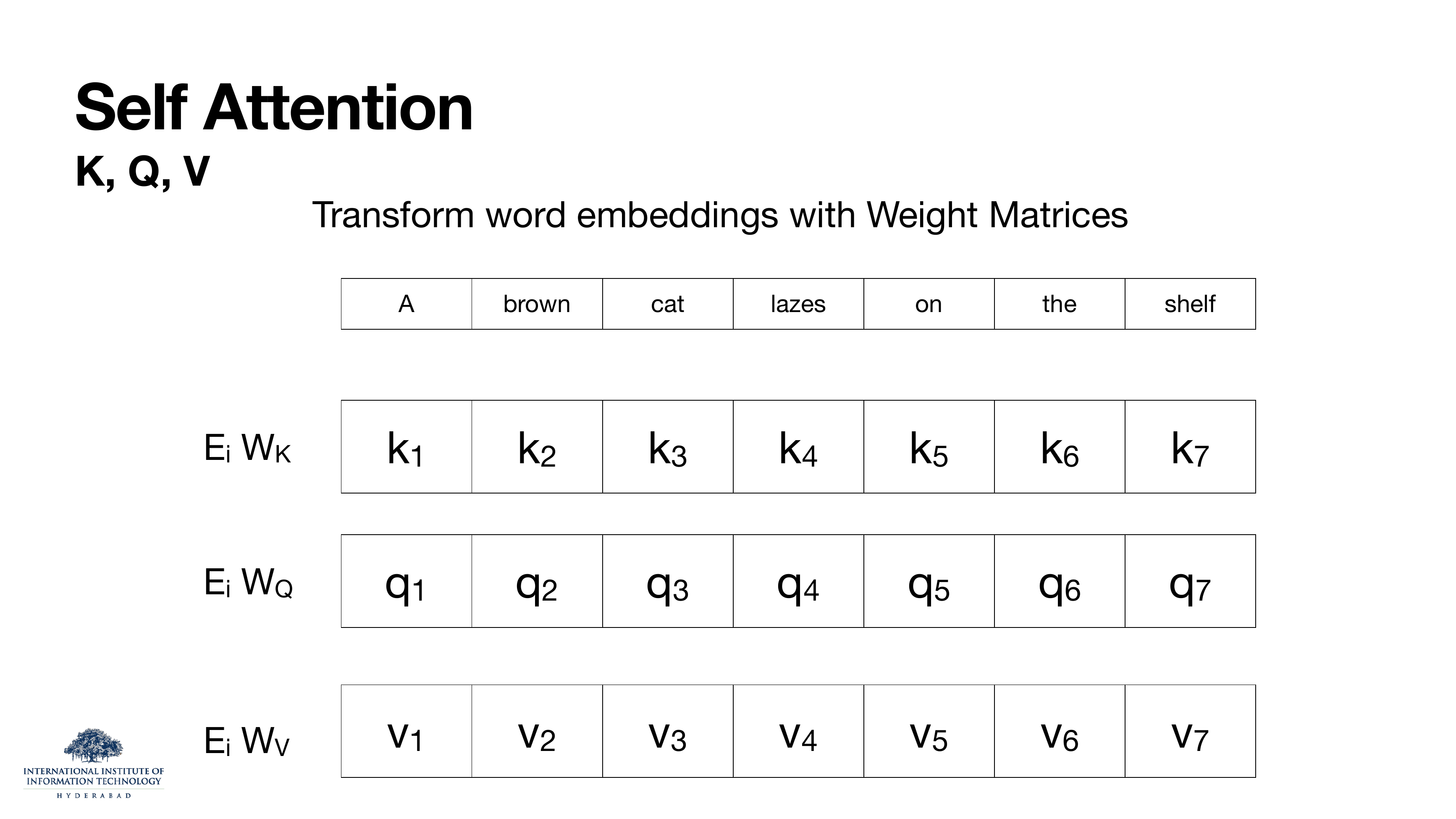
On these slides

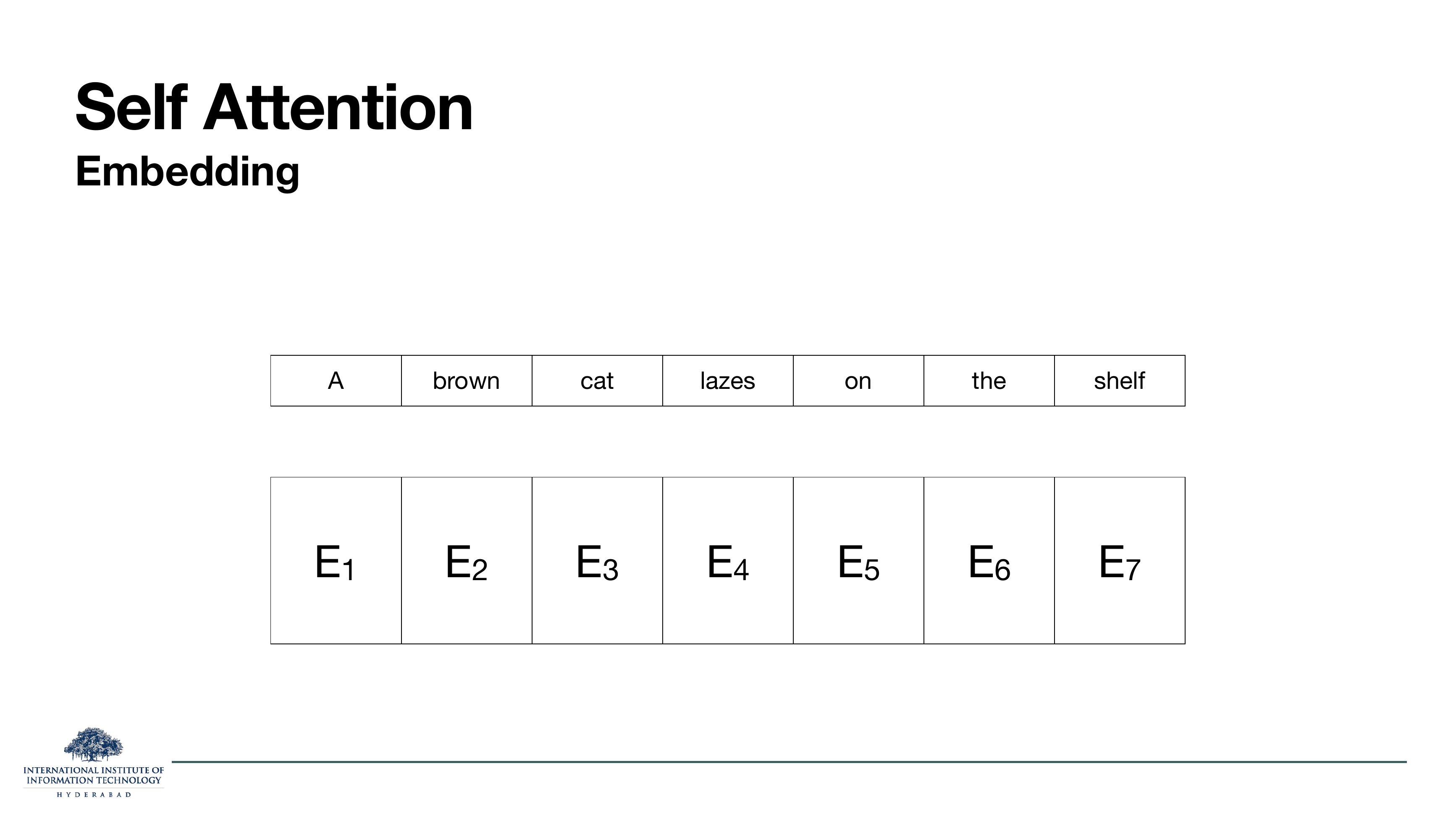
Three snapshots of the same construction. Each token starts as an embedding E_i. Three learned linear projections, W_Q, W_K, W_V, turn that one embedding into three role-specific vectors:

Query q_i: "here is what I am looking for."
Key k_i: "here is what I contain."
Value v_i: "here is what I will hand over if I get picked."

The database analogy is exact: a query is compared against every key, the resulting scores decide who wins, and the winner's value is returned. Only softer, instead of one winner we take a weighted average of all values.

Slide 57 / 90

Attention matrix cells filled with scaled dot products QK^T / sqrt(d_k). Normalize with sqrt(d) for stability.

slide 57 · dot products

Slide 58 / 90

After softmax: q_3 ('cat') row shows attention weights 0, 0.38, 0.48, 0.08, 0.01, 0, 0.05 over A/brown/cat/lazes/on/the/shelf.

slide 58 · softmax

Slide 59 / 90

Multiply the softmaxed weights by V — the row for 'cat' averages the value vectors weighted by 0/0.38/0.48/...

slide 59 · weighted sum of values

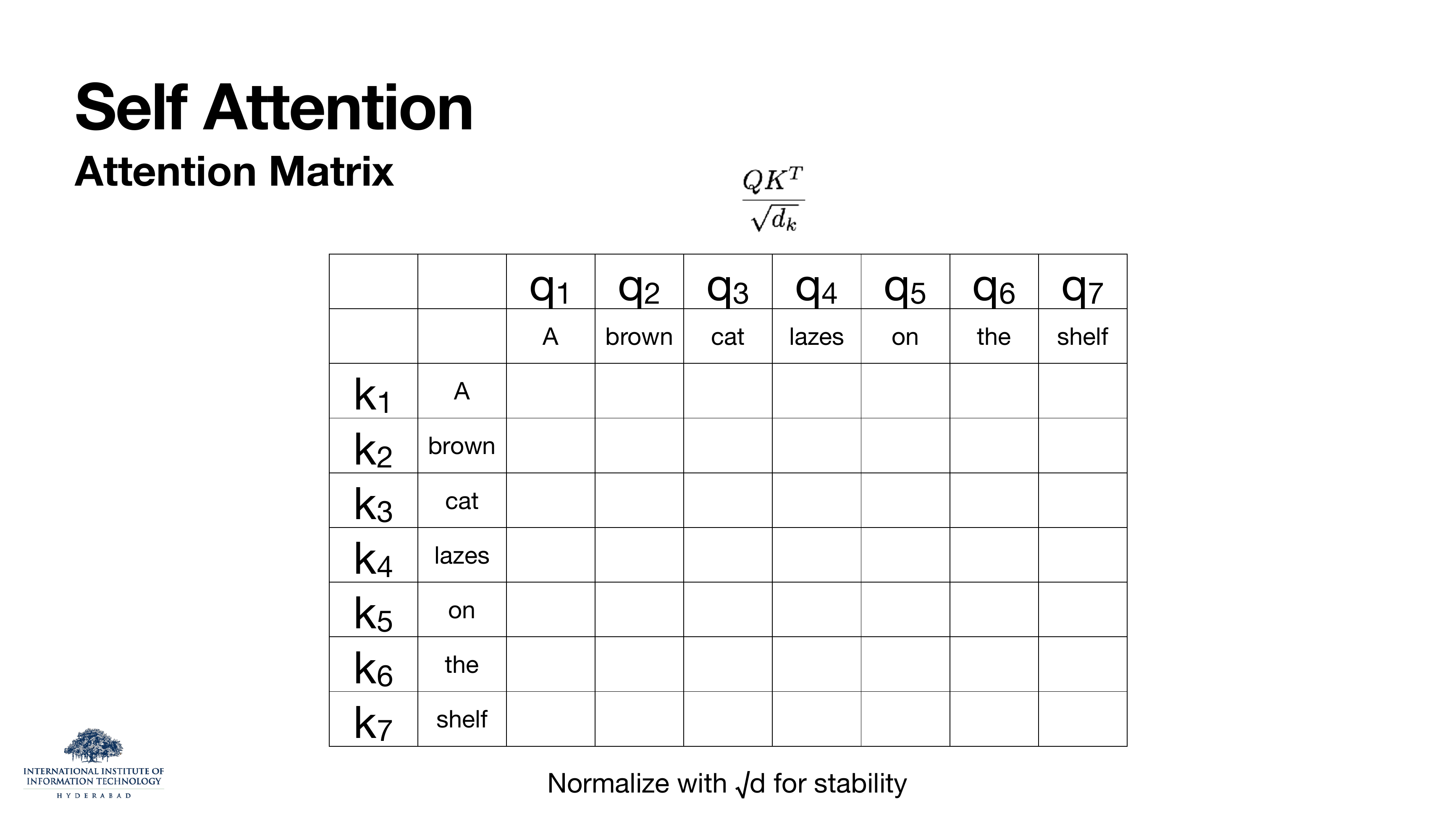
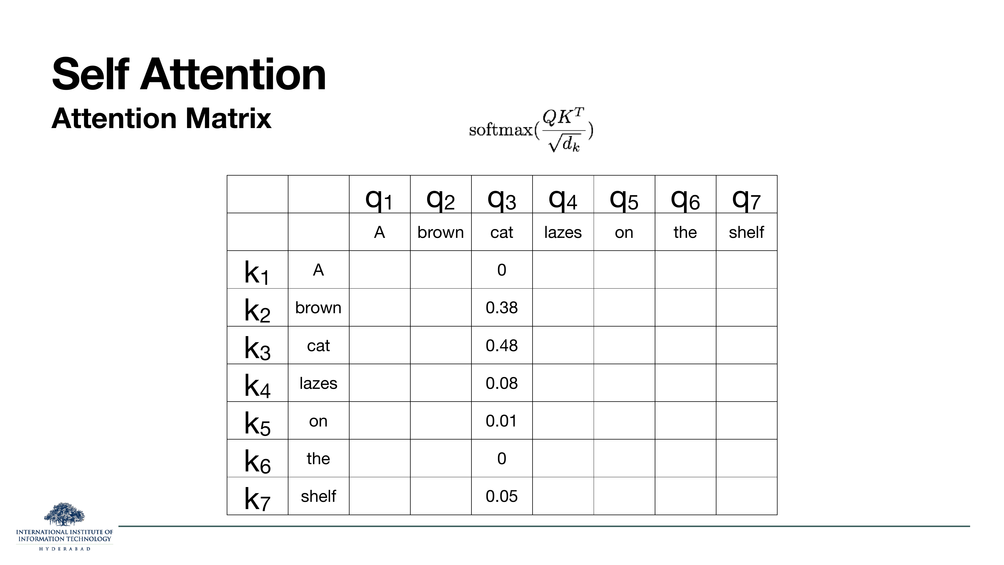
On these slides

The formula on slide 53, worked column by column for the query q₃ (the word "cat"). Slide 57 fills the column with scaled dot products. Slide 58 softmaxes them into a distribution (numerical example: 0.38 on "brown", 0.48 on "cat" itself, 0.08 on "lazes", small mass elsewhere). Slide 59 uses that distribution to weight-average the value vectors.

✦ Key takeaway

Read the numbers on slide 58 carefully. The output representation for "cat" ends up as roughly 0.48 × v(cat) + 0.38 × v(brown) + a smaller piece of v(lazes). That is precisely what "the embedding of cat should absorb the adjectives that modify it" looks like in code.

Slide 60 / 90

Same formula Attention(Q,K,V)=softmax(QK^T/sqrt(d_k)) V shown again as a reminder before the matrix picture.

slide 60 · formula recap

Slide 61 / 90

Shapes: X is n × d_embed. W_Q, W_K are d_embed × d_k, giving Q, K of shape n × d_k. W_V is d_embed × d_v, giving V of shape n × d_v.

slide 61 · the shapes

On these slides

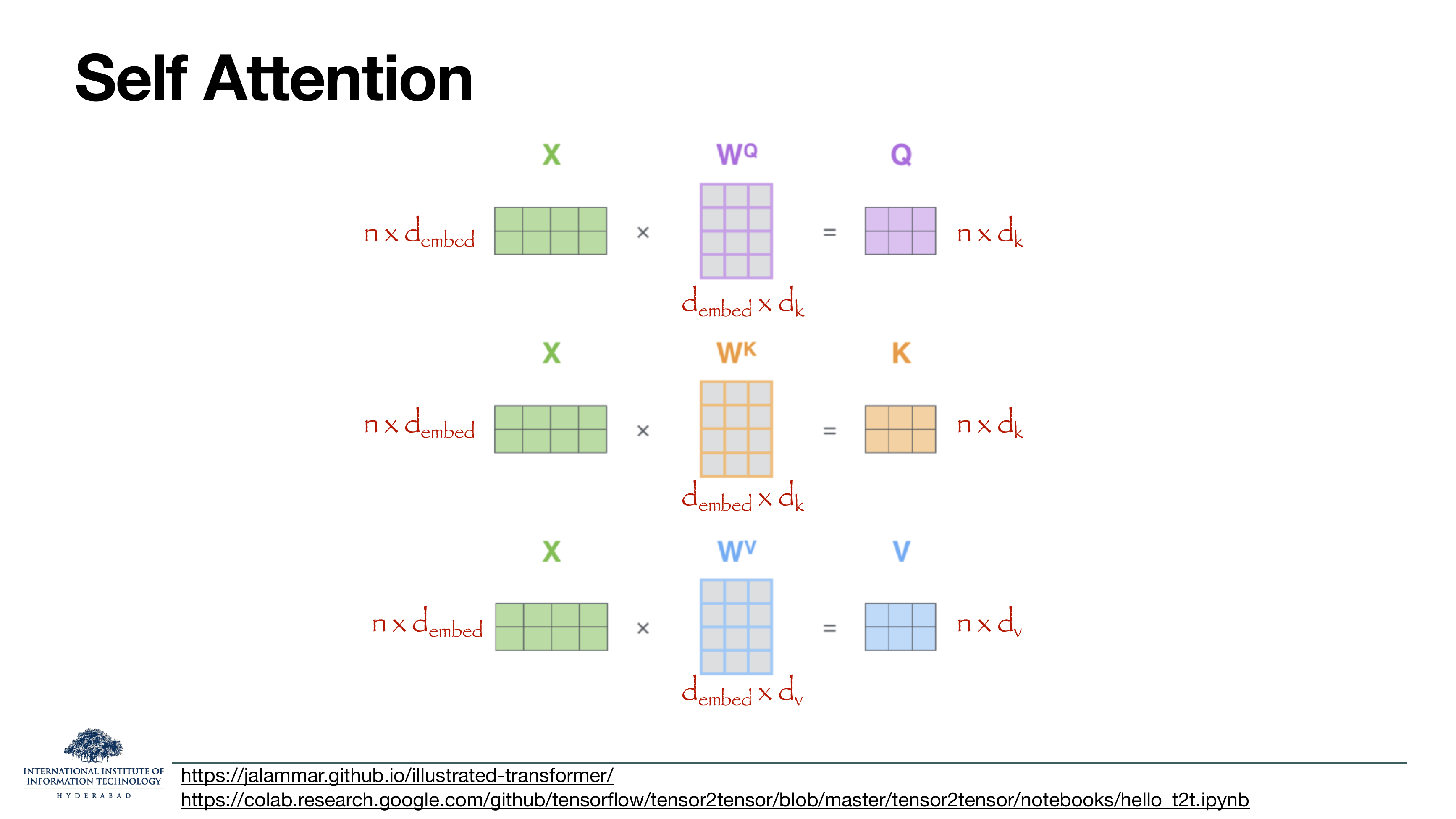
The same operation as a matrix multiply. X is an n×d_embed input (all tokens stacked as rows). Three projection matrices W_Q, W_K, W_V take X to Q, K, V. The whole self-attention layer is now three matrix multiplies, one softmax, and one more matrix multiply. Every step is a single GPU kernel, and every position is computed at the same time.

✦ Key takeaway

This is why the transformer is fast. Compare with an RNN: n sequential steps, each depending on the previous one. Self-attention: two matrix multiplies, no sequence. The trade is that the attention matrix has n×n entries, so cost is O(n²×d). For short-to-medium sequences that is a win; for very long ones it is the pain point the "More Attention" lecture will address.

Slide 62 / 90

Multi-Head Attention: (1) input sentence, (2) embed each word, (3) split into 8 heads and multiply X or R with weight matrices, (4) calculate attention using resulting Q/K/V matrices per head, (5) concatenate the Z matrices then multiply with W^O to produce the layer output.

slide 62 · eight parallel heads

On the slide

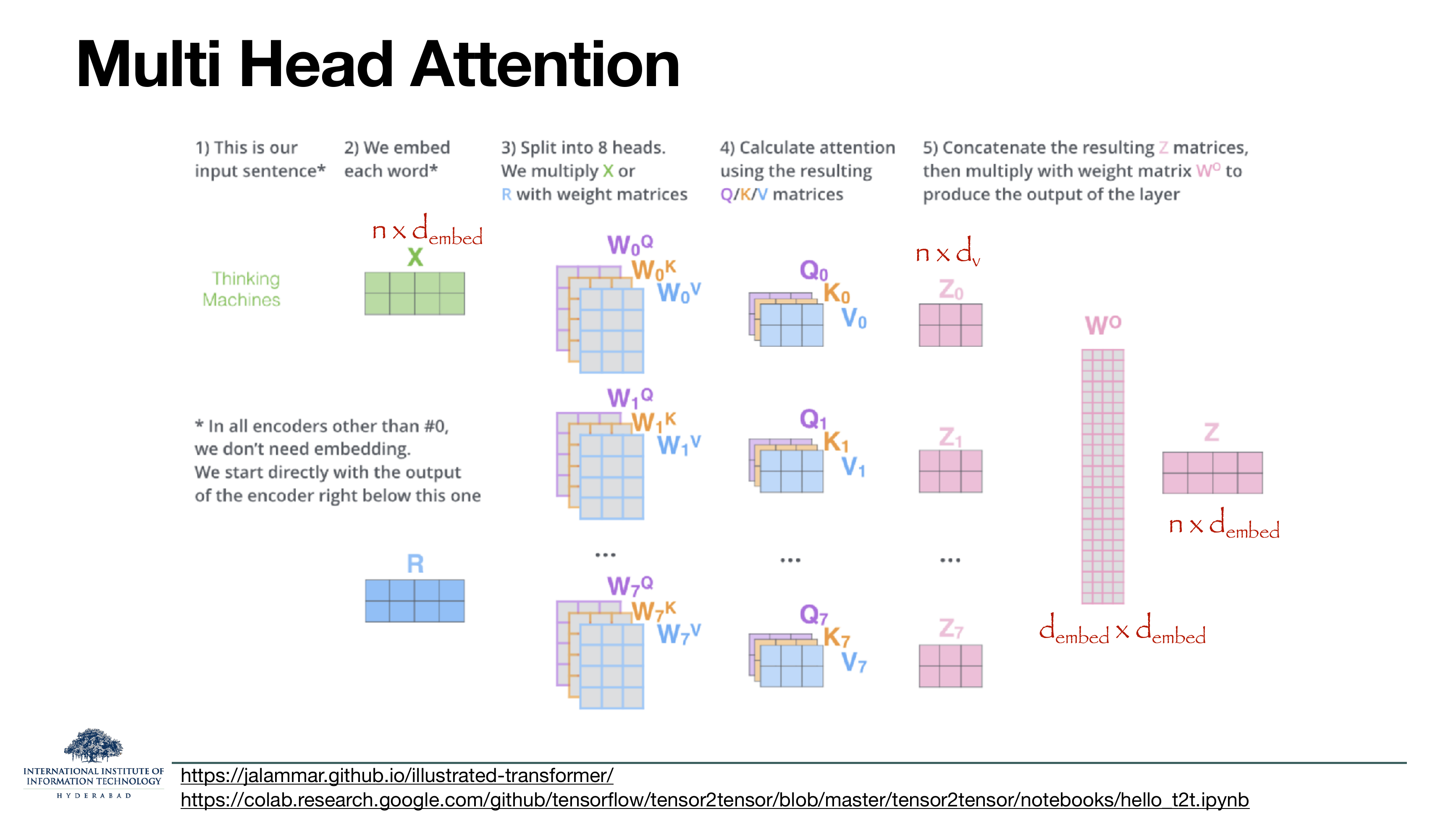
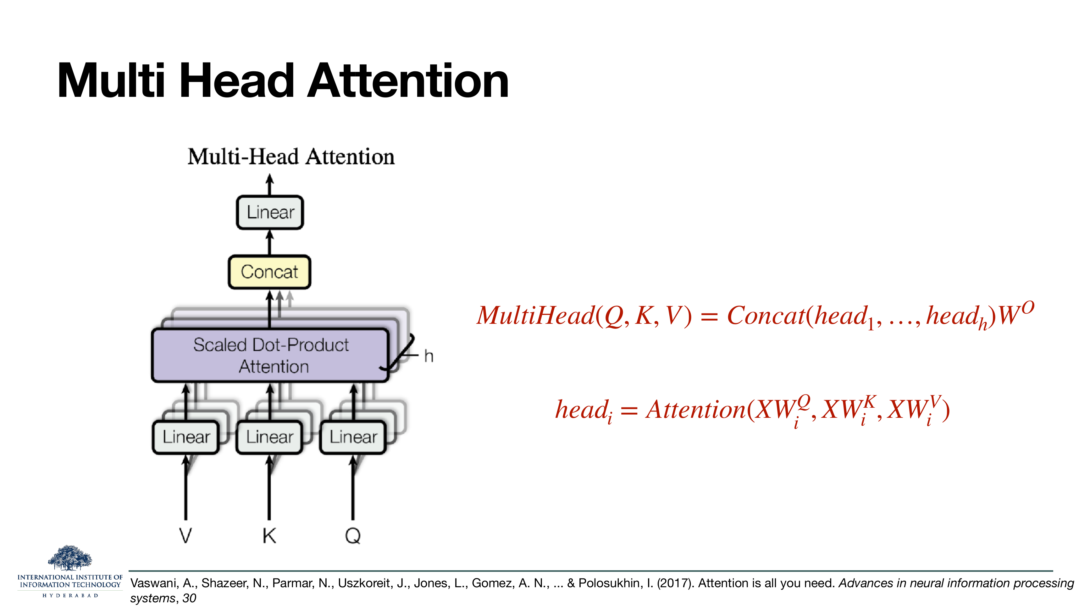
The transformer runs attention h times in parallel (the paper picked h=8); each head has its own W_Q, W_K, W_V triple. Every head produces its own output matrix Z_i. Those matrices are concatenated along the feature axis and passed through a final output projection W^O.

Why multiple heads

One attention distribution can only pay attention to one kind of relationship at a time. If it is busy resolving "it → animal", it cannot also be tracking "cross → street". Multiple heads let the layer represent many relationship types simultaneously at the same layer, each in its own low-dimensional subspace.

Slide 63 / 90

Scaled Dot-Product Attention block from Vaswani et al.: Q and K go into MatMul, output is scaled, optionally masked, softmaxed, then multiplied by V. head_i = softmax((XW_Q_i)(XW_K_i)^T / sqrt(d_k) + AttentionMask)(XW_V_i).

slide 63 · scaled dot-product block

Slide 64 / 90

Multi-Head Attention block: V, K, Q each go through a Linear, then h scaled dot-product attention blocks in parallel, then concat, then a final Linear. MultiHead(Q,K,V) = Concat(head_1,...,head_h) W^O.

slide 64 · multi-head block

On these slides

The two figures from the paper. Slide 63 zooms in on one head; note the optional attention mask added before the softmax, which is how the decoder gets to hide future tokens from itself during training. Slide 64 stacks h of those heads, concatenates, and applies the output projection W^O.

Under the hood

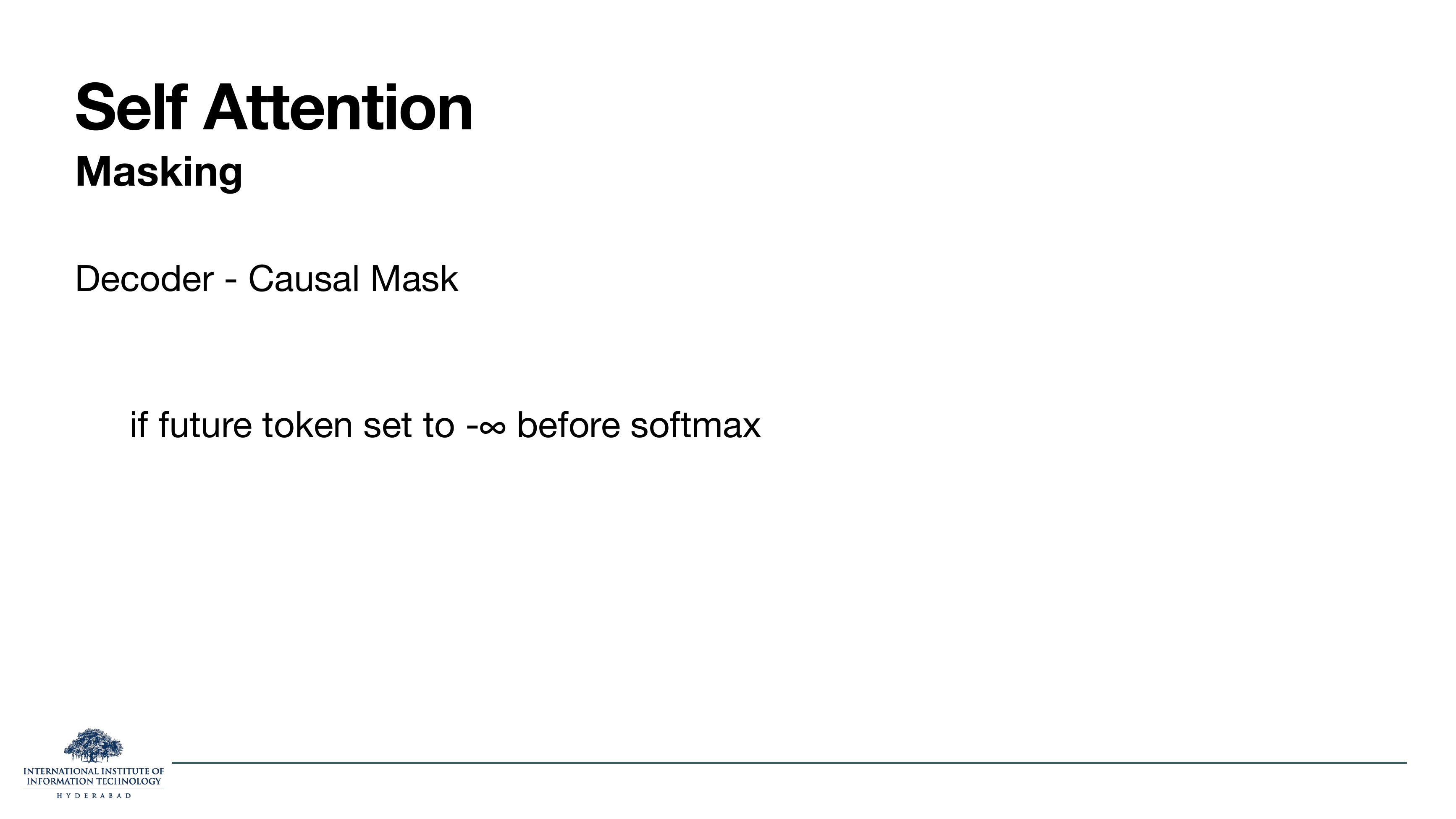
The mask is just a matrix of the same n×n shape as QK^T, with a value of −∞ wherever you want to hide a position and 0 elsewhere. Adding −∞ before the softmax makes that cell exactly zero afterwards. In a causal (decoder-side) transformer, the mask is upper-triangular: every position is blocked from looking at future positions.

Slide 65 / 90

Self-Attention Gains: computational complexity per layer (faster than RNN when seq len n < d, the representation dimensionality); parallelization; long distance dependency.

slide 65 · why we switched

On the slide

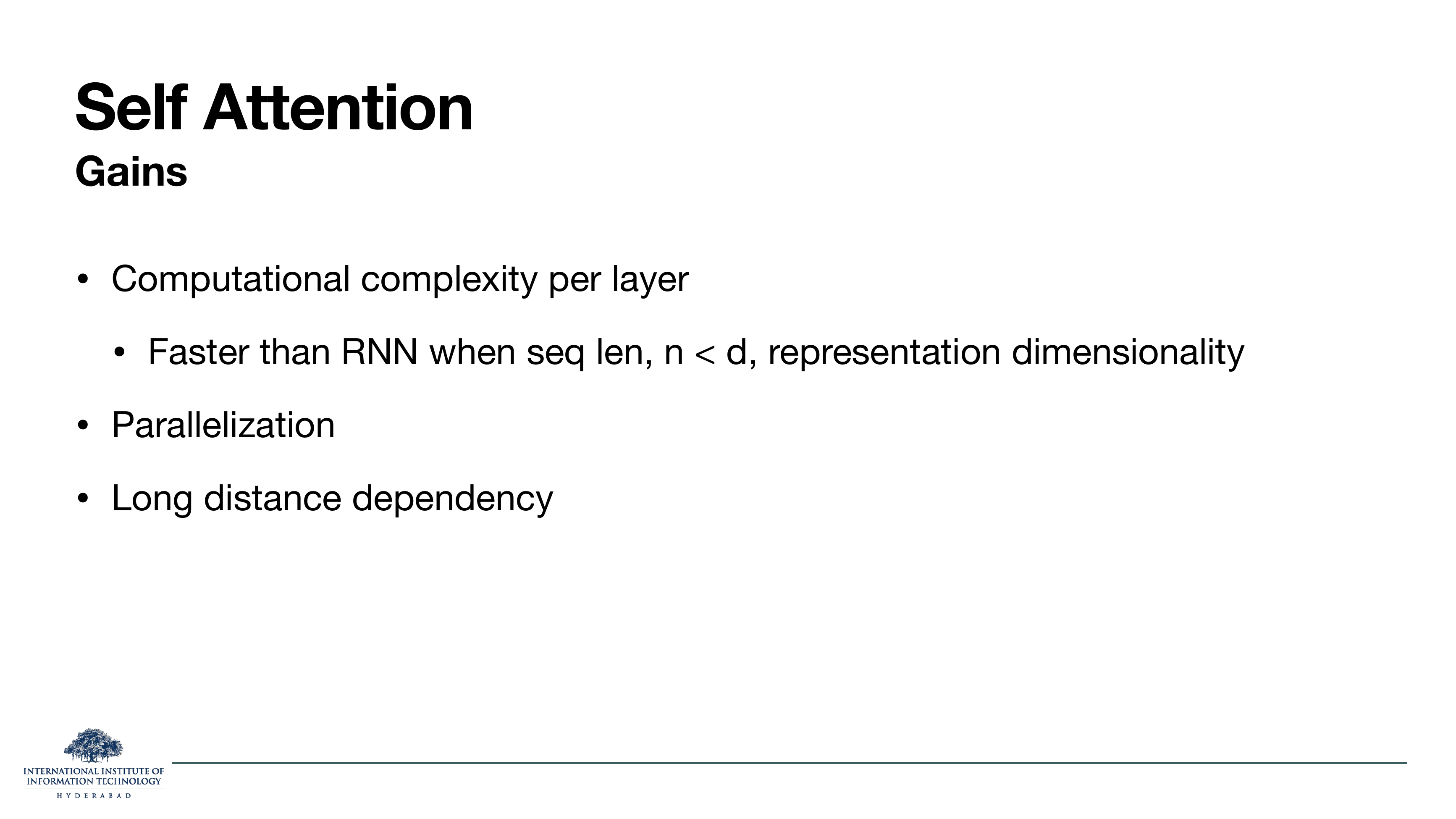
The scorecard. Self-attention wins on all three axes that killed the RNN.

Computational complexity per layer. O(n² d) for self-attention vs. O(n d²) for an RNN. Self-attention is faster whenever n < d, which is the regime almost every serious deep model runs in.
Parallelisation. Every position is a matrix-multiply row, computable in parallel. No unrolled loop.
Long-distance dependency. Any two positions are one attention hop apart. No gradient product to vanish.

→ Keep reading

The one thing self-attention does not do out of the box is know about order. The next section fixes that.

§8Position, non-linearity, masking, block

Ten slides. Now that we have raw self-attention, the deck lists what is still missing and adds one small piece at a time until the picture matches Figure 1 of the paper. Positional encoding for order, the feed-forward network for non-linearity, causal masking for the decoder, and finally residual connections plus layer norm so the whole thing trains.

Slide 66 / 90

Self-attention missing: no word position, no non-linearity, looks at future words.

slide 66 · what's missing

On the slide

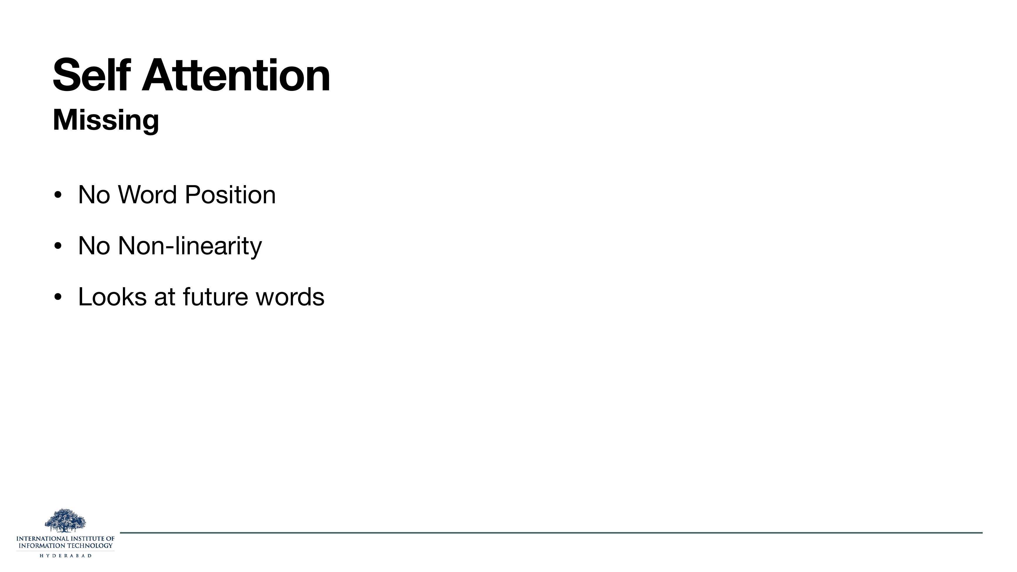
Three problems with raw self-attention.

No word position. Swap "dog bites man" for "man bites dog" and every attention score stays the same, the model is permutation-invariant.
No non-linearity. Self-attention is a weighted sum of linear projections. Stacking pure attention layers still gives you a linear function.
Looks at future words. A language-model decoder must not see word t+1 when predicting word t. Vanilla self-attention peeks freely.

Slides 67 through 71 address each of these in turn.

Slide 67 / 90

Positional encoding: PE(pos,2i) = sin(pos / 10000^(2i/d_model)), PE(pos,2i+1) = cos(pos/10000^(2i/d_model)). Diagram shows the PE vector added to token embeddings for 'Je suis étudiant'.

slide 67 · the formula

Slide 68 / 90

Positional encoding: 'Sinusoidal positional encoding may allow the model to extrapolate to sequence lengths longer than the ones encountered during training.'

slide 68 · why sinusoids

Slide 69 / 90

Positional encoding heatmap: 20 tokens on the y-axis, 512 embedding dimensions on the x-axis, coloured by PE value. Left half generated by sines, right half by cosines.

slide 69 · what it looks like

On these slides

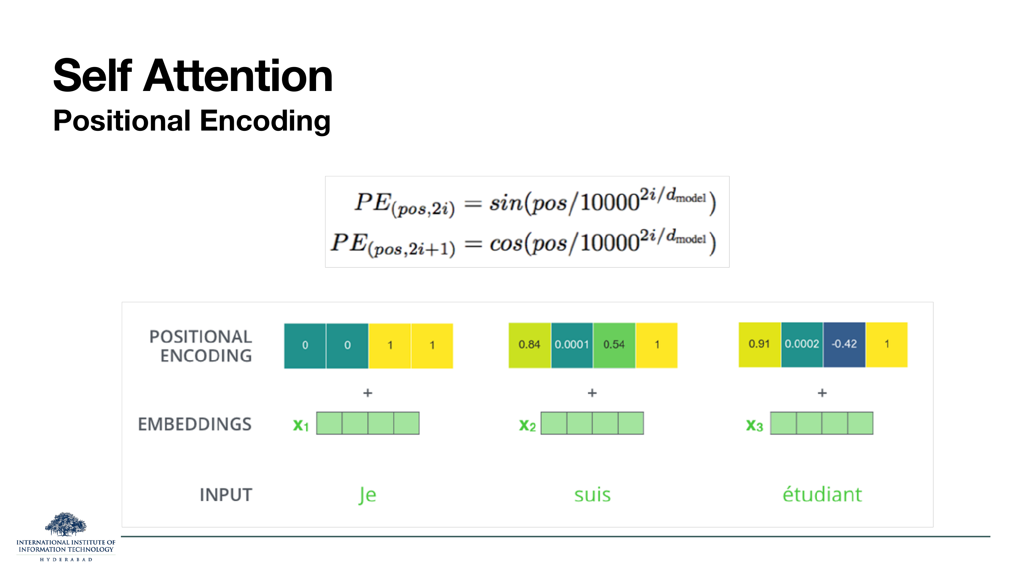
The sinusoidal positional encoding from the paper.

\begin{matrix} {PE}_{(pos, 2 i)} & = \sin (pos / 10000^{2 i / d_{model}}) \\ {PE}_{(pos, 2 i + 1)} & = \cos (pos / 10000^{2 i / d_{model}}) \end{matrix}

Each position pos gets a vector the same size as the token embedding, made of sines and cosines at geometrically decreasing frequencies. That vector is added to the token embedding before it enters the first attention layer.

✦ Key takeaway

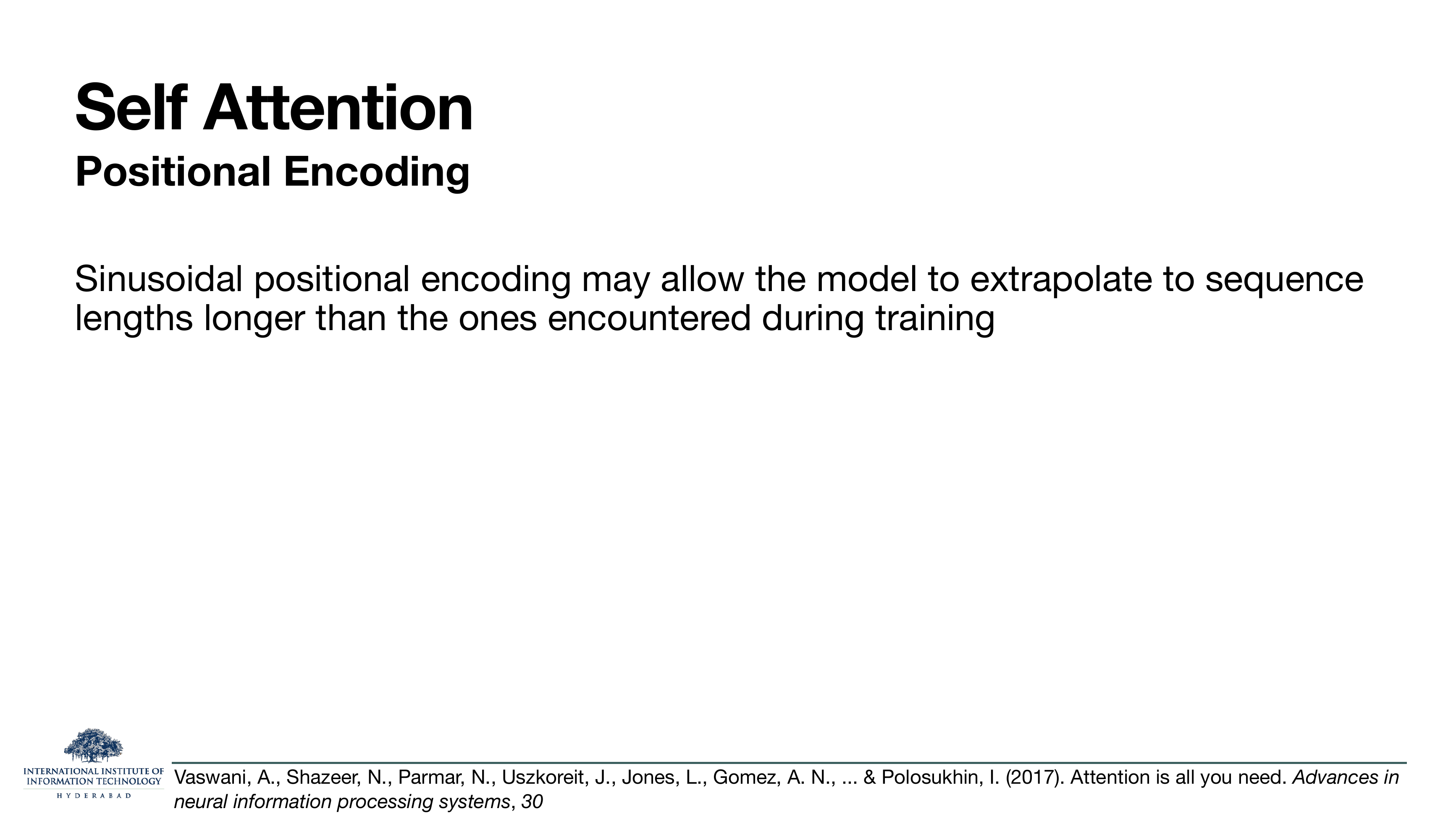
Why sinusoids? Because sin(a+b) and cos(a+b) can be written as linear combinations of sin(a), cos(a), sin(b), cos(b). So the model can learn a linear operator that says "shift by k positions", and that operator will work for any k, including k's longer than any position seen during training. That is the "extrapolate to longer sequences" claim on slide 68.

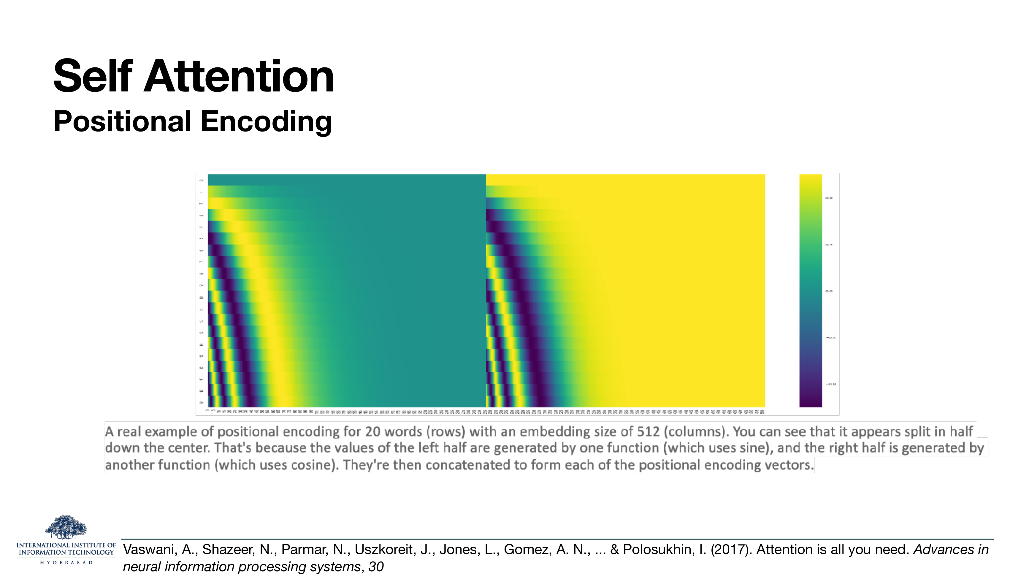
Slide 69 is the visualisation everyone remembers: 20 positions on the vertical, 512 embedding dims on the horizontal, sines on the left half of the vector, cosines on the right, frequencies falling as you go right. Each row is a unique fingerprint for that position.

→ Keep reading

Modern transformers usually replace sinusoidal PE with RoPE (rotary position embeddings) or ALiBi. See the "positional encoding" lecture later in the course. But sinusoids remain the textbook default and are still what LLaMA-style diagrams draw.

Slide 70 / 90

Self-Attention Non-Linearity: feed forward neural network to process every layer.

slide 70 · FFN for non-linearity

On the slide

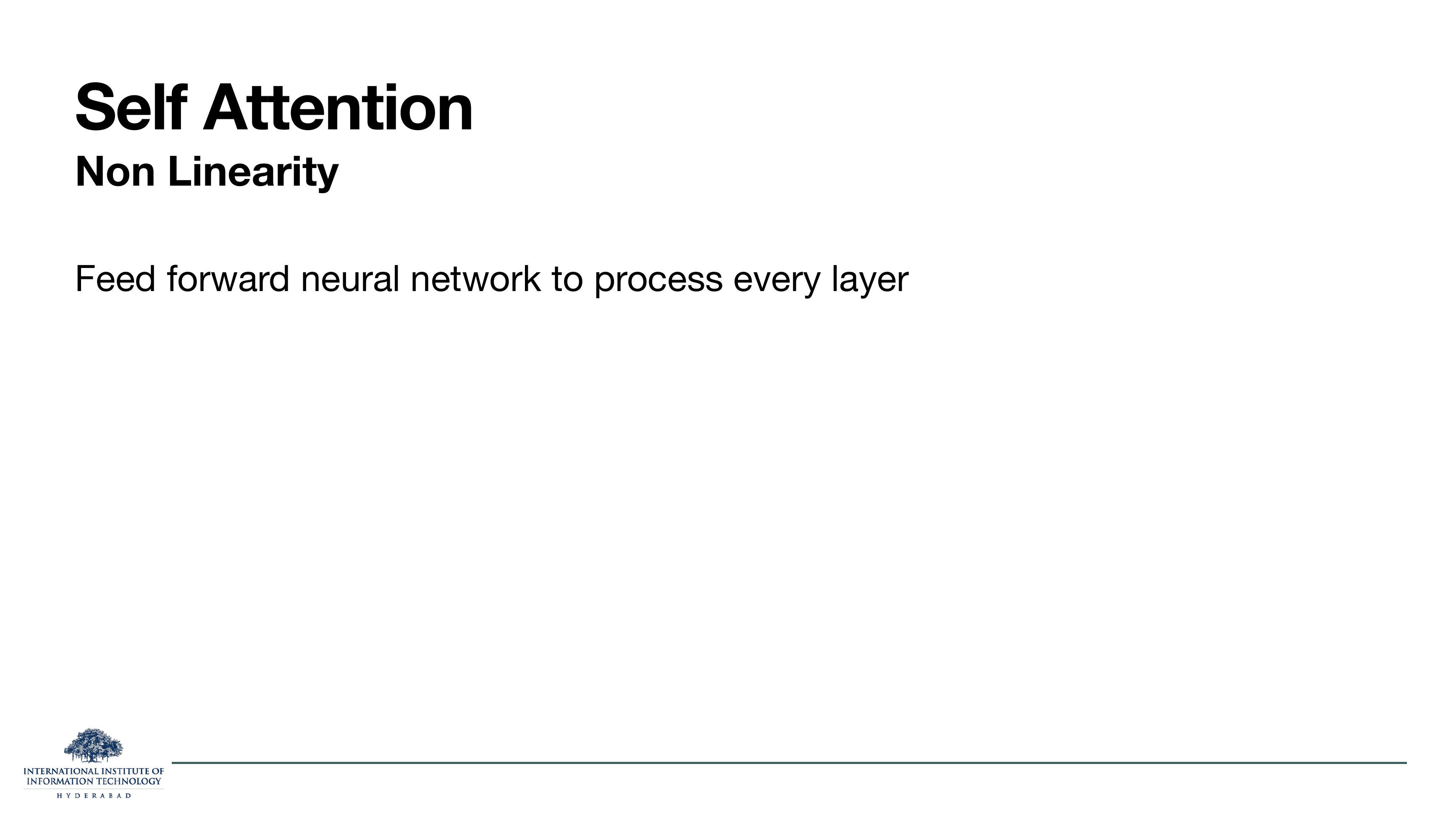
The fix for "no non-linearity": after every attention layer, add a small position-wise feed-forward network, a two-layer MLP applied independently to every token, with a ReLU (or GeLU) in the middle.

FFN (x) = max (0, x W_{1} + b_{1}) W_{2} + b_{2}

This is where most of the parameter count of a modern transformer actually lives, the FFN's hidden dimension is typically 4× the model dimension.

Slide 71 / 90

Self-attention masking: decoder causal mask, if future token set to -infinity before softmax.

slide 71 · causal mask

On the slide

The fix for "looks at future words". In the decoder, before the softmax, we add a matrix that is 0 on the lower triangle and −∞ on the upper triangle. After softmax those −∞ entries become zero, so no position can attend to a later one.

Under the hood

This is called causal masking. It is the one architectural difference between an encoder-only model (BERT, no mask, every position sees every other position) and a decoder-only model (GPT, causal mask, each position sees only its predecessors).

Slide 72 / 90

Transformer Encoder block: Input Embedding + Positional Encoding → Multi-Head Attention → Add & Norm → Feed Forward → Add & Norm, repeated Nx.

slide 72 · encoder block

Slide 73 / 90

Transformer Decoder block: Output Embedding + Positional Encoding → Masked Multi-Head Attention → Add & Norm → Multi-Head Attention (cross) → Add & Norm → Feed Forward → Add & Norm, repeated Nx, then Linear + Softmax to output probabilities.

slide 73 · decoder block

On these slides

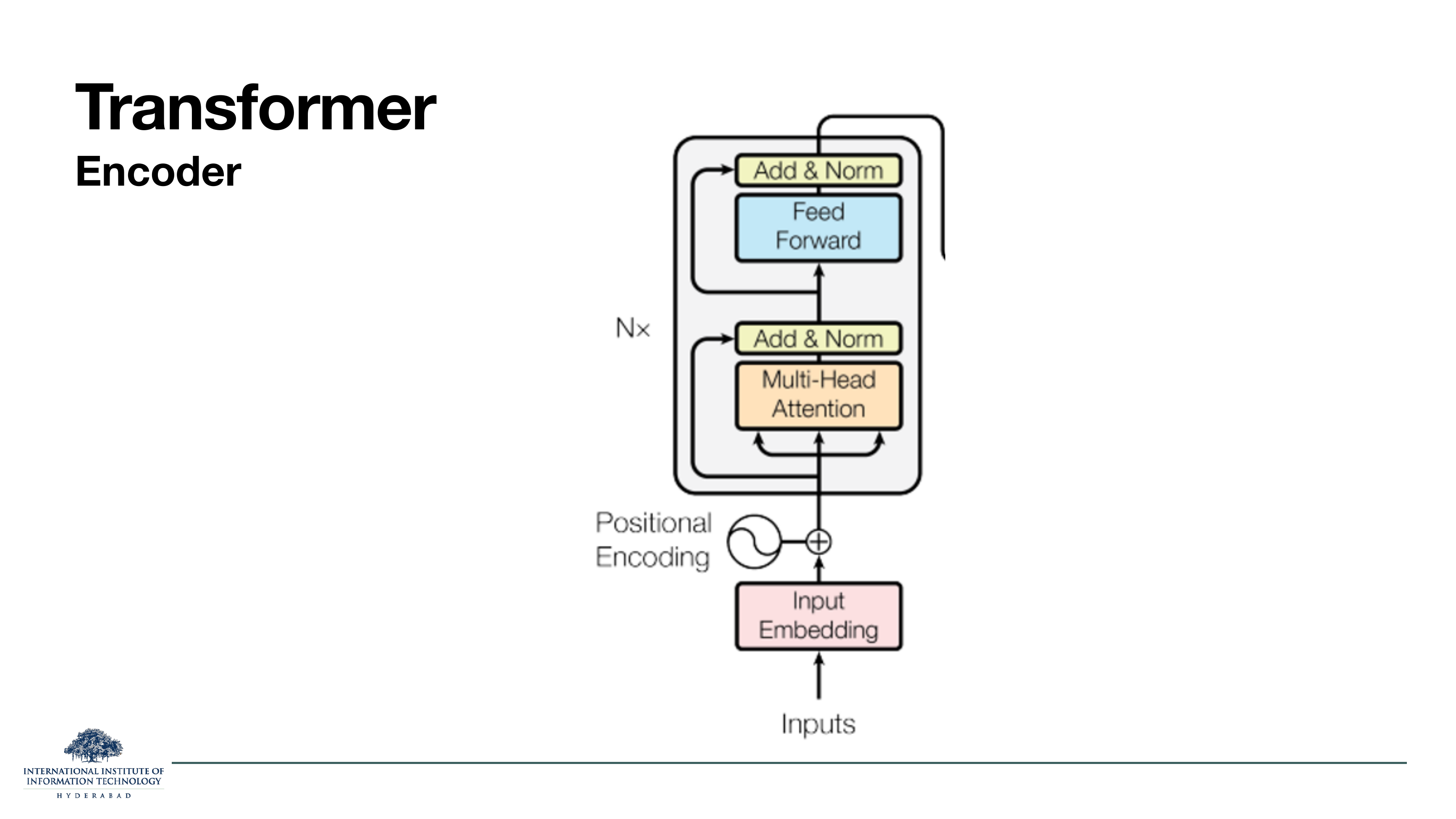
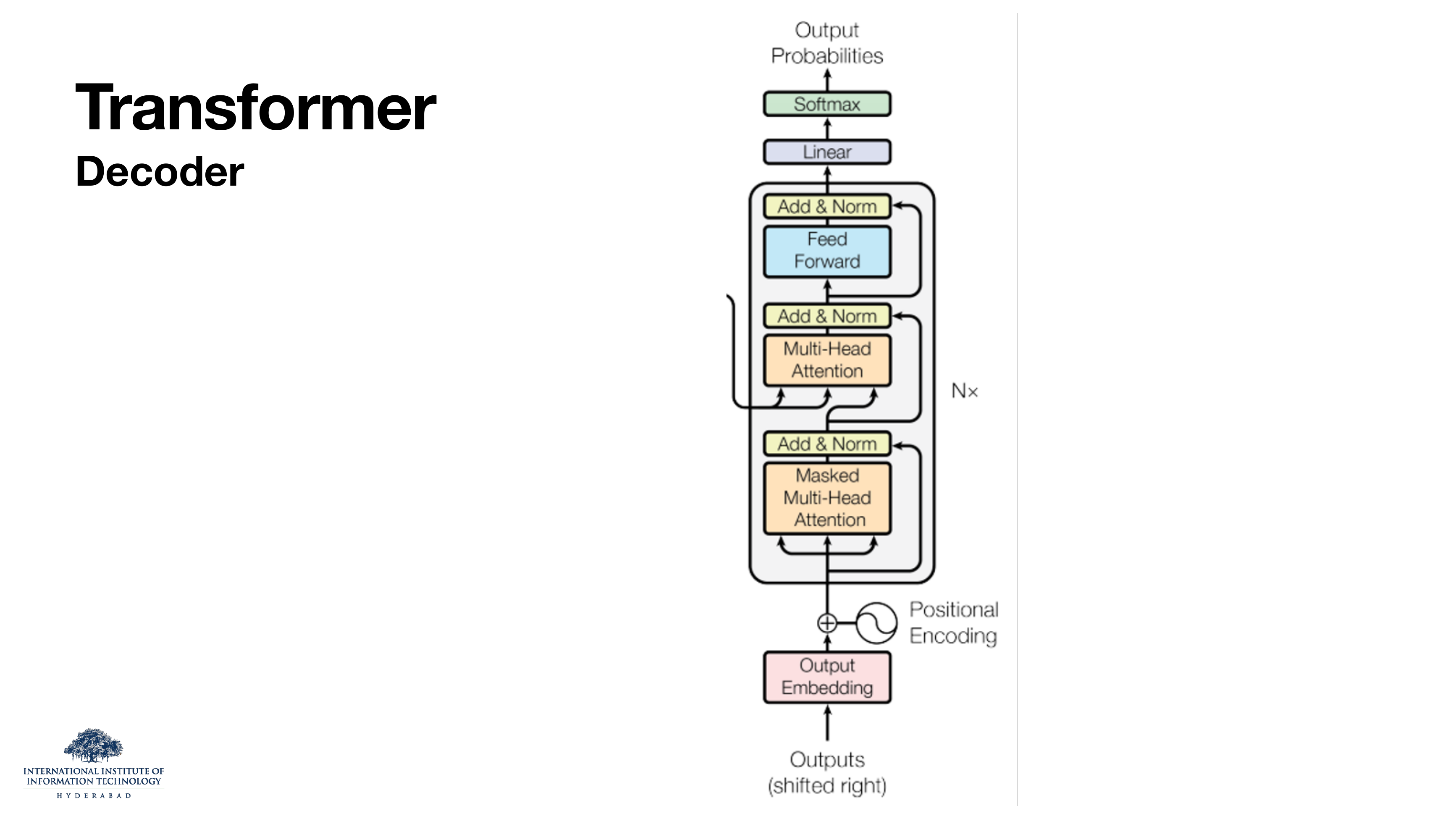
Everything from the last five slides, wired into a single block. The encoder block: input embedding + positional encoding, then N repetitions of (multi-head self-attention → Add & Norm → feed-forward → Add & Norm).

The decoder block adds two things: (a) the first attention sublayer is masked, and (b) a second attention sublayer sits on top, which is cross-attention: its queries come from the decoder, but its keys and values come from the encoder output. That is how the decoder actually reads the source sentence.

✦ Key takeaway

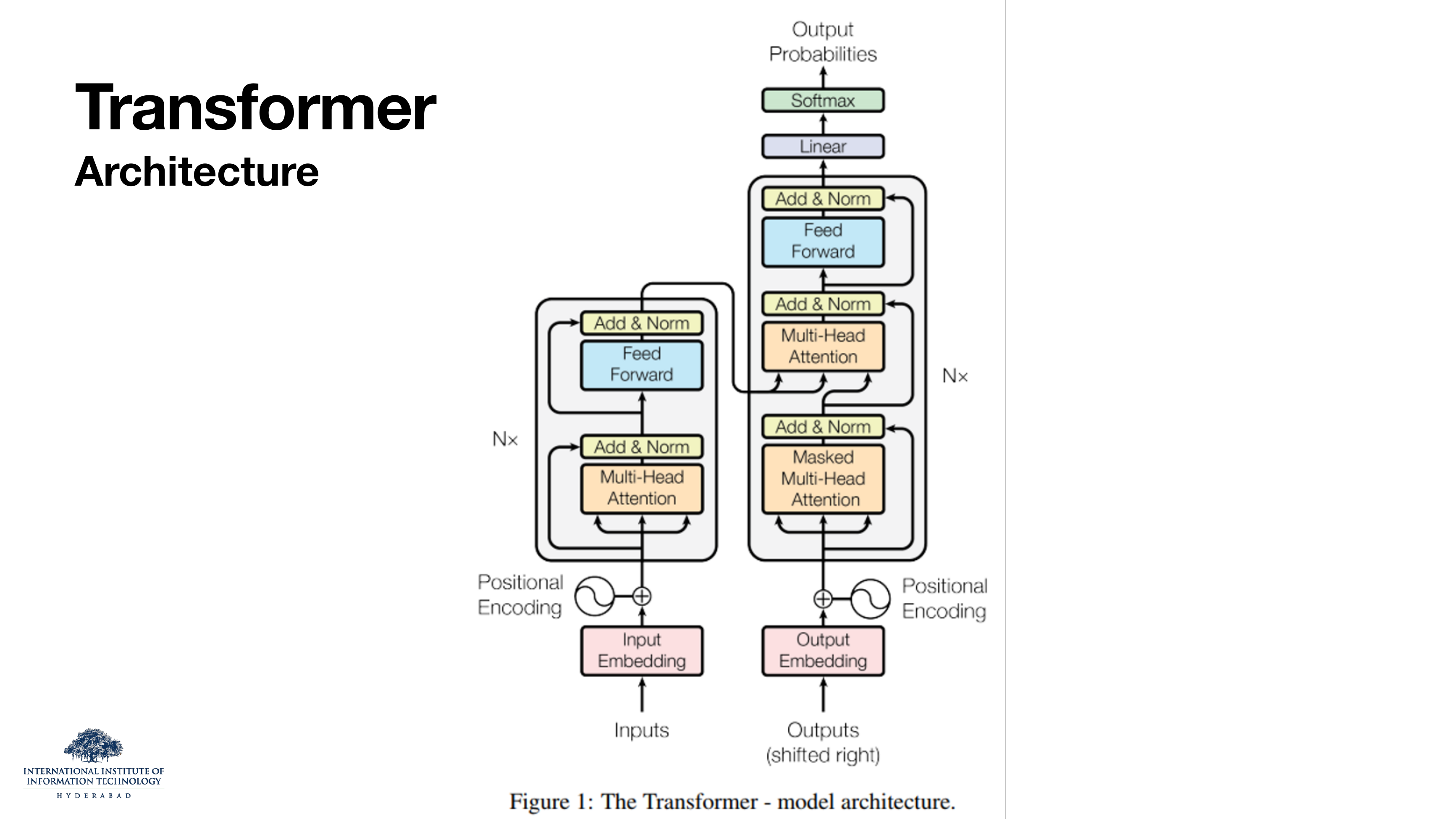
The Bahdanau attention from slides 41-44 is exactly the cross-attention sublayer on slide 73. What was a bolt-on to the RNN in 2015 is now one of three attention sublayers per decoder block. The transformer did not invent attention, it noticed you could use it everywhere.

Slide 74 / 90

Transformer Architecture: the full encoder–decoder diagram from Vaswani et al. Figure 1, with encoder on the left, decoder on the right, and cross-attention arrows from encoder output into the decoder's second attention sublayer.

slide 74 · the whole diagram

Slide 75 / 90

Add and Layer Normalization: residual connections (train better, smooth loss function); layer norm (normalize to unit mean and s.d. in each layer, cuts down uninformative variation).

slide 75 · Add & Norm

On these slides

Slide 74 is Figure 1 of Attention Is All You Need: encoder on the left, decoder on the right, cross-attention arrows in the middle. This is the diagram of the field. Being able to redraw it from memory is one of the things this whole deck is training you to do.

Slide 75 zooms in on the two yellow "Add & Norm" boxes that appear all over the diagram.

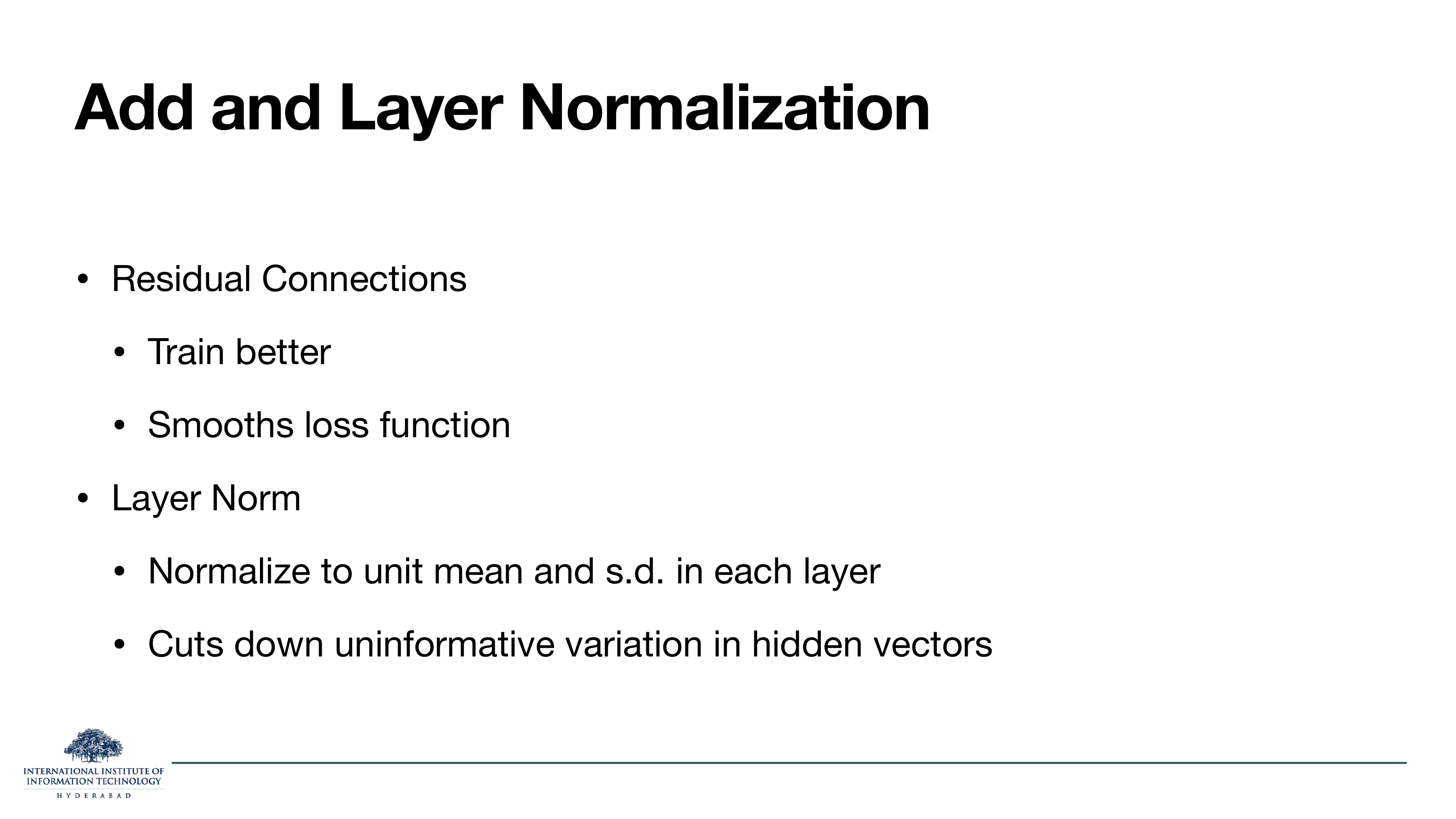
Residual (skip) connection: the sublayer's output is added to its input. This gives the gradient a shortcut path all the way back to the first layer. Without residuals, transformers deeper than a few layers do not train at all.
Layer normalisation: inside each token vector, rescale to zero mean and unit variance, then multiply by learned gain and add learned bias. This keeps activations in a well-behaved range as they pass through many layers.

Under the hood

Layer norm normalises across the feature dimension of one token, not across the batch (that is batch norm) or across positions (that is instance norm). Because it never mixes information between positions, it plays cleanly with variable sequence lengths, which is precisely what sequence models need.

§9The transformer, seen whole

Nine slides. The lecture zooms out and asks: given the block we just built, what actually flows through it, what does each parameter cost us, and where does the architecture still hurt? This is the section where you get a feel for the shape of a modern transformer: the tensors, the parameter counts, the trade-offs the next nine lectures will attack.

Slide 76 / 90

Residual Connection: the loss surface of ResNet-56 (a) without skip connections is chaotic and jagged; (b) with skip connections is smooth and bowl-shaped.

slide 76 · why residuals

On the slide

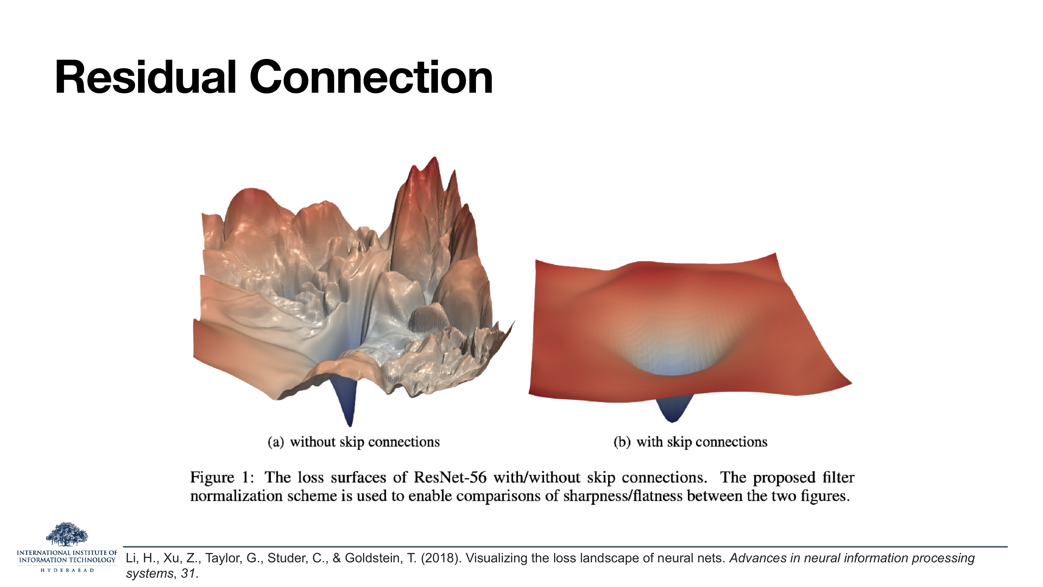
Two loss landscapes for ResNet-56, from Li et al. 2018. Without skip connections the loss surface is a chaotic mountain range full of sharp peaks and saddles; with them it is a smooth bowl with a single global minimum.

✦ Key takeaway

This picture is why the "Add" in "Add & Norm" is not decorative. Residual connections do not just help gradients flow, they geometrically reshape the loss surface into something an optimiser can actually walk down. Take them out and a 100-layer transformer would not train.

Slide 77 / 90

Types of Attention: encoder self-attention (arcs among tokens in one sequence), encoder-decoder attention (arcs from a decoder token to all encoder tokens), masked decoder self-attention (arcs only to previous decoder tokens).

slide 77 · three flavours of attention

On the slide

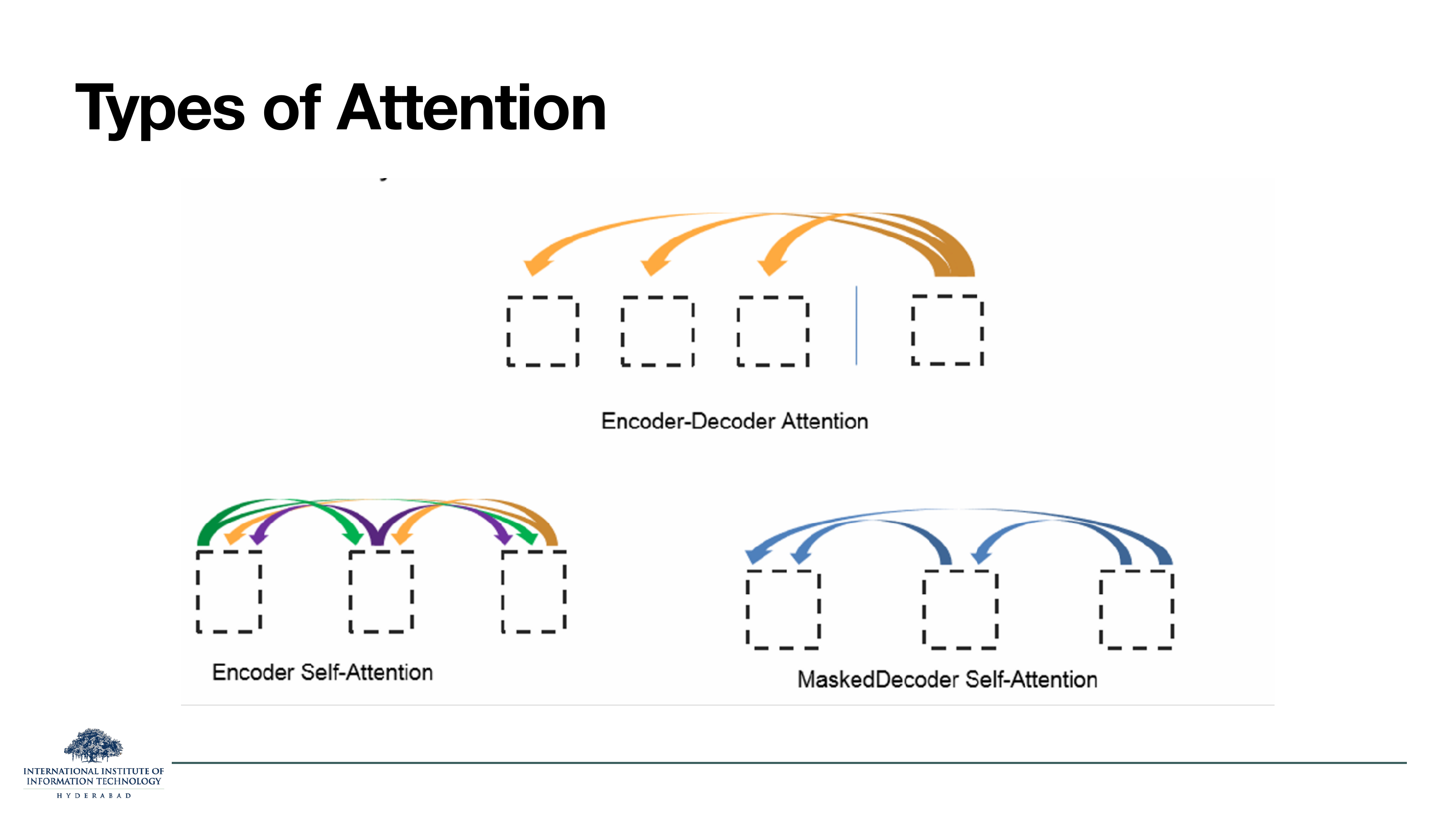
The three places attention appears in a full encoder-decoder transformer.

Encoder self-attention: every source token attends to every source token.
Encoder-decoder (cross) attention: each decoder token attends to every encoder token.
Masked decoder self-attention: each decoder token attends to prior decoder tokens only.

Same equation, different Q/K/V sources and different mask.

Slide 78 / 90

Cross Attention: Encoder-Decoder Attention — decoder vectors as Q, encoder output as K and V. Every word in decoder looks for possible words from encoder. Two distinct types of data: machine translation, speech to text.

slide 78 · cross attention

On the slide

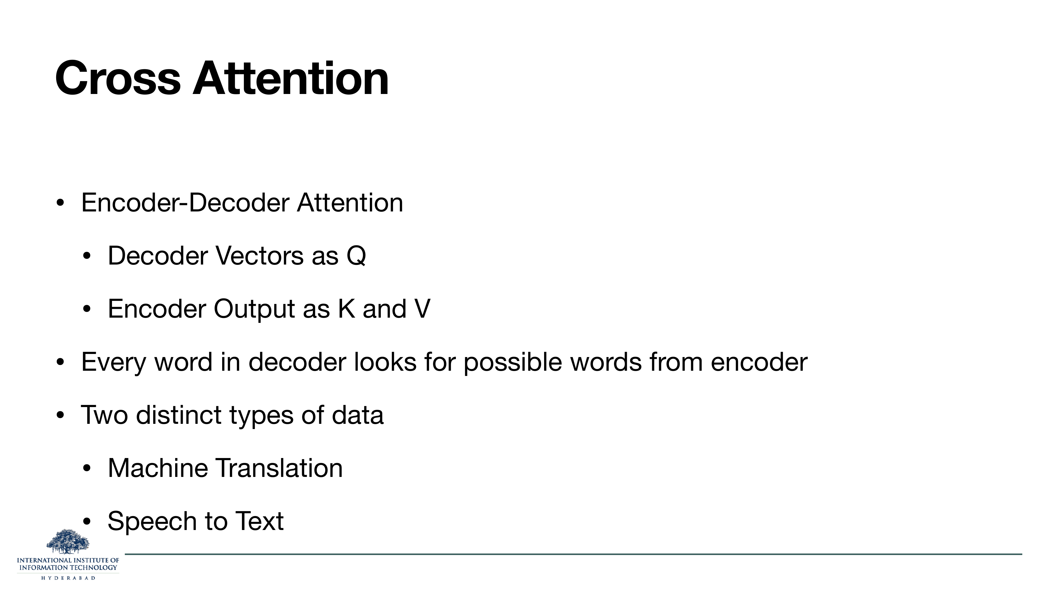
The exact wiring of cross-attention: queries come from the decoder, keys and values come from the encoder's output. This is what lets the decoder "read" the source.

→ Keep reading

Cross-attention is not just for translation. It is the mechanism behind any two-tower model: an image encoder feeding a text decoder (image captioning), an audio encoder feeding a text decoder (speech-to-text, Whisper), a retrieved-document encoder feeding a generator (Fusion-in-Decoder). Learn the pattern once, use it everywhere.

Slide 79 / 90

Transformer Gains: parallel processing, semi-supervised learning, transfer learning, knowledge-stores, reasoning.

slide 79 · what the transformer bought us

Slide 80 / 90

Transformer Drawbacks: quadratic computation in self-attention, position representation.

slide 80 · what it still hurts on

On these slides

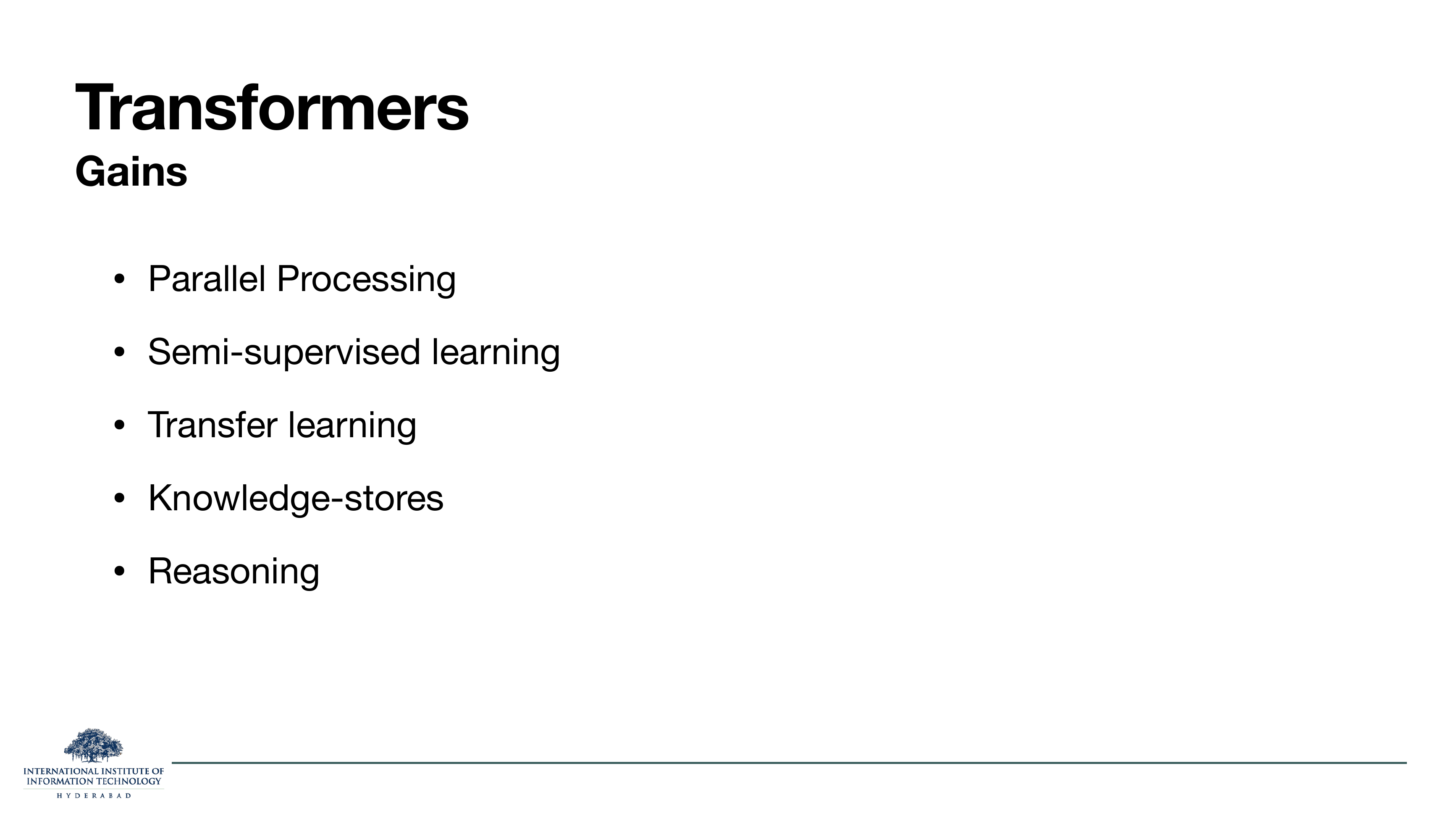
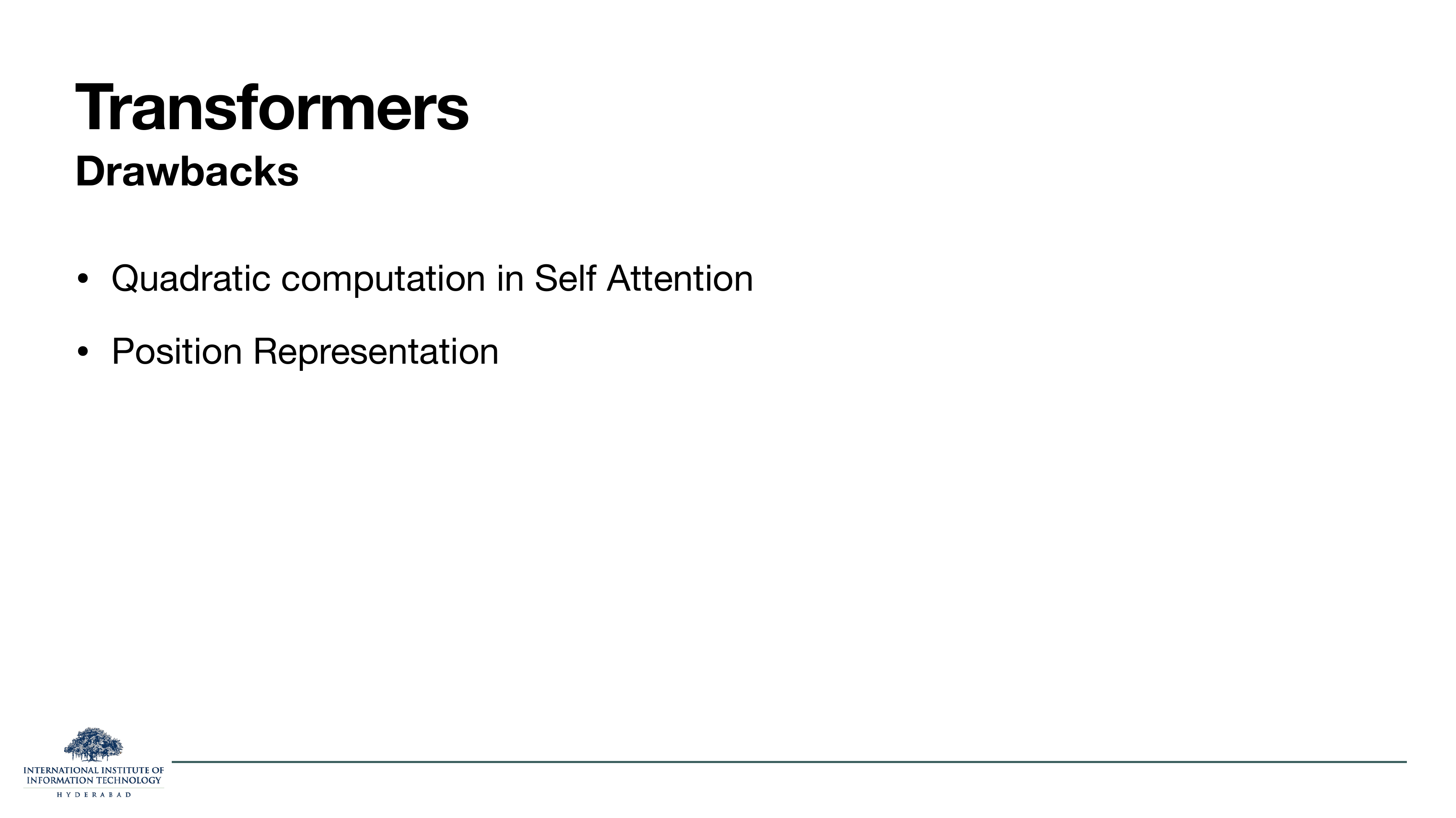
Five wins, two pain points. Slide 79 lists the wins:

Parallel processing at training time (the reason "train on the whole internet" ever became feasible).
Semi-supervised learning and transfer learning: pretrain on next-token prediction, fine-tune on anything.
Knowledge stores: the FFN layers act as key-value memory, storing facts.
Reasoning: chain-of-thought and its descendants exploit the depth of attention layers.

Slide 80 names the two open wounds: (1) the attention matrix is O(n²) in sequence length, and (2) positional encoding is a bolt-on that never quite settles.

Slide 81 / 90

Transformer Advances in position representation: learned representations, relative position representations, absolute position, Rotary Position Embeddings (RoPE), NoPE.

slide 81 · position fixes

Slide 82 / 90

Transformer Advances in attention: sparse attention, grouped query attention, multi head latent attention, log linear attention, linear attention.

slide 82 · attention fixes

On these slides

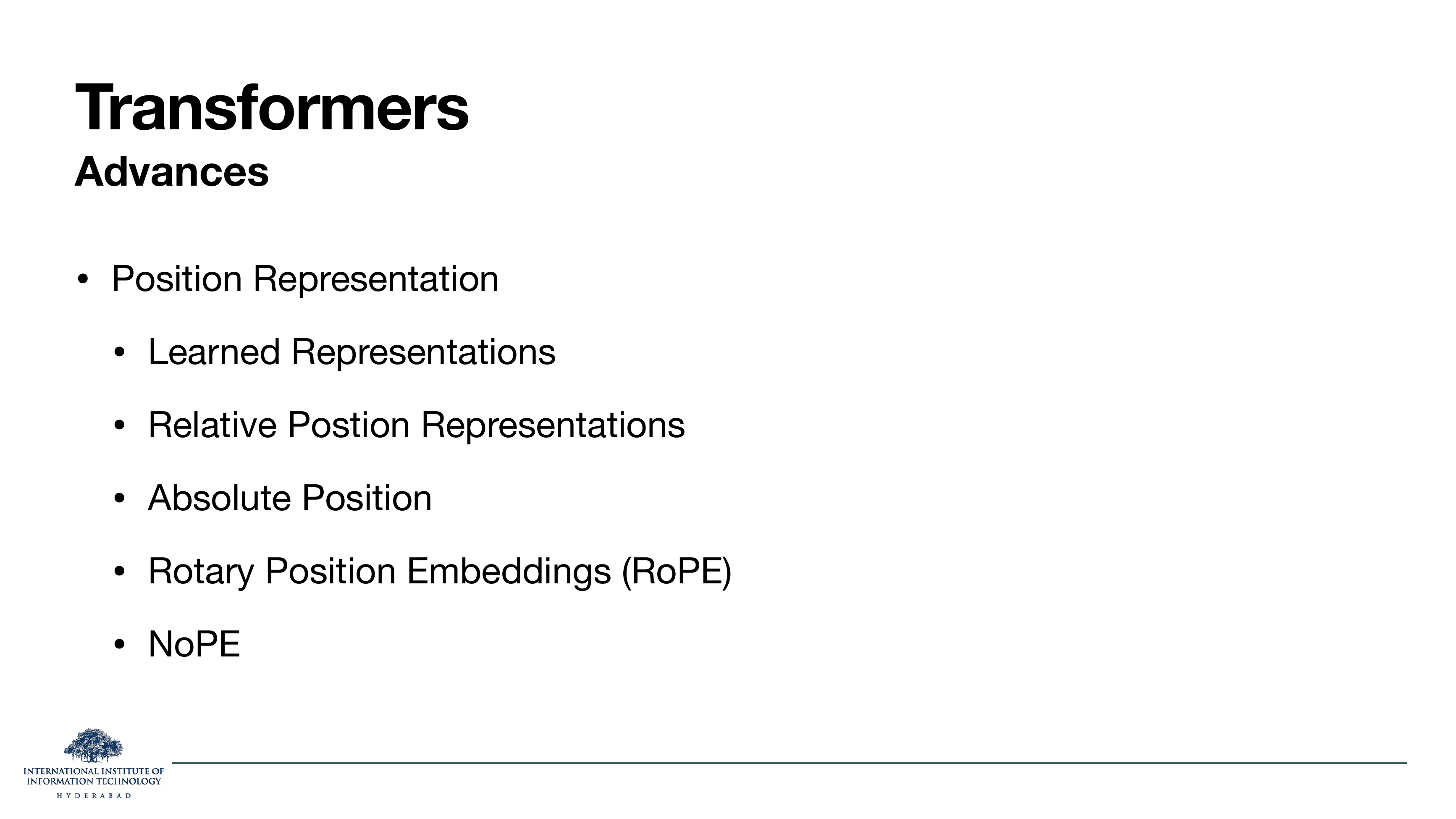
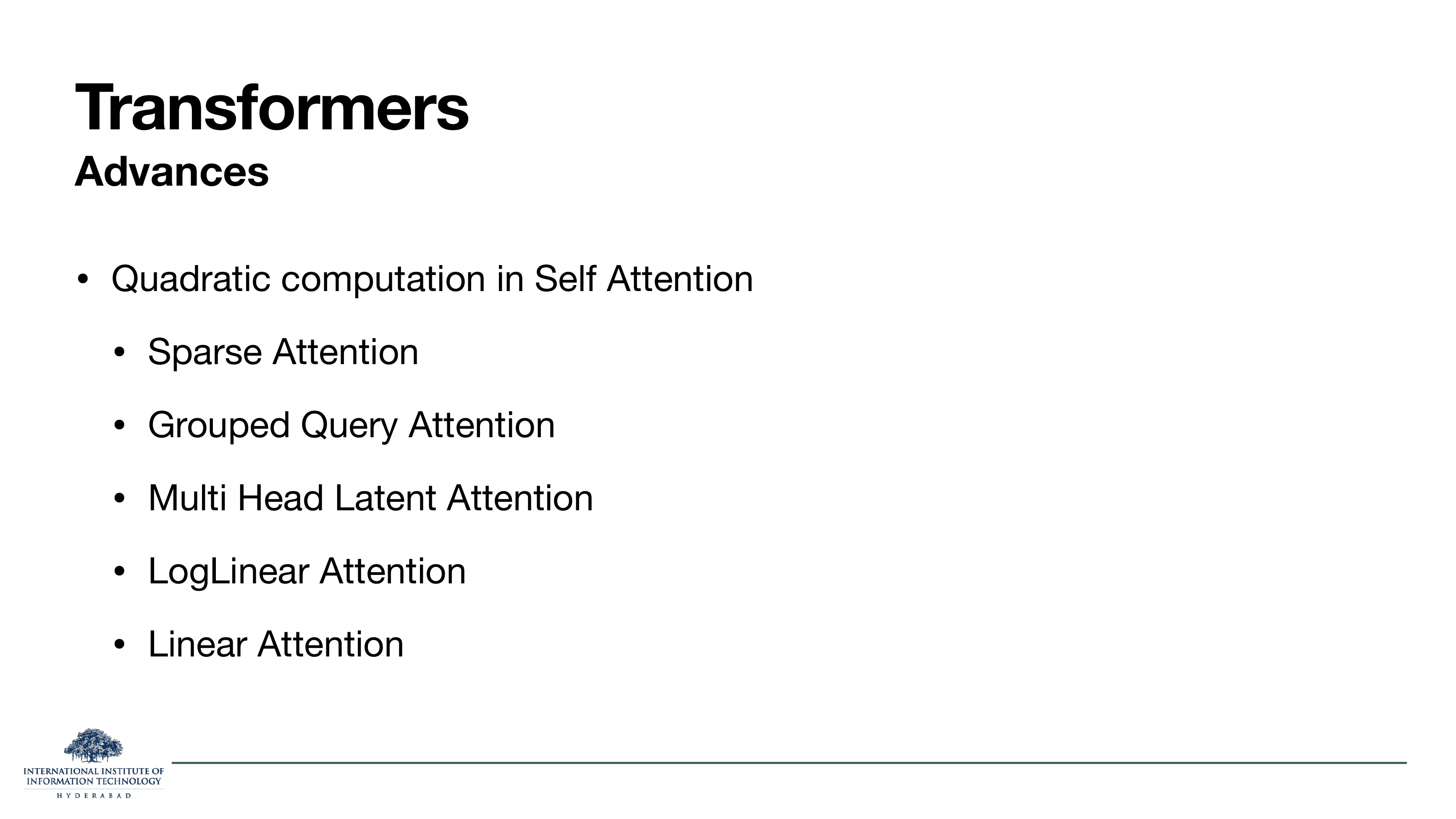
The two open problems in slide 80, each with a shopping list of research responses.

Position: learned, relative, absolute, RoPE (rotary position embeddings, the LLaMA default), and even NoPE (no positional encoding at all, letting causal masking do the work).
Attention efficiency: sparse attention (only compute a subset of the matrix), grouped-query attention (share K/V across heads, LLaMA-2, Mistral), multi-head latent attention (DeepSeek-V2's trick), log-linear and linear attention (algorithmic escapes from the n² cost).

→ Keep reading

Every one of these gets its own lecture later: More Attention covers sparse, grouped-query, and Flash Attention; the positional-encoding lecture covers RoPE and NoPE; the alternate-architectures block covers state-space models as the more radical version of "linear attention".

Slide 83 / 90

Transformer Shape: block diagram of Embedding → Pre Norm → Attention → Post Norm → FFNN → Final Norm → Output. Shapes: token embedding V×d, Q/K/V heads×n×d, W_up d×4d, W_down 4d×d, output d×V.

slide 83 · shapes of every tensor

Slide 84 / 90

Parameter counts for a ~1B model: V=32000, d=2048, n=2048, dq=128, h=l=16. Token embedding 65M (7%), positional 4.2M (0.4%), attention 268M (29%), FFN 536M (57%), decoding 65M (7%), bias/layer norm 0.3M. Total 935.8M.

slide 84 · where the parameters live

On these slides

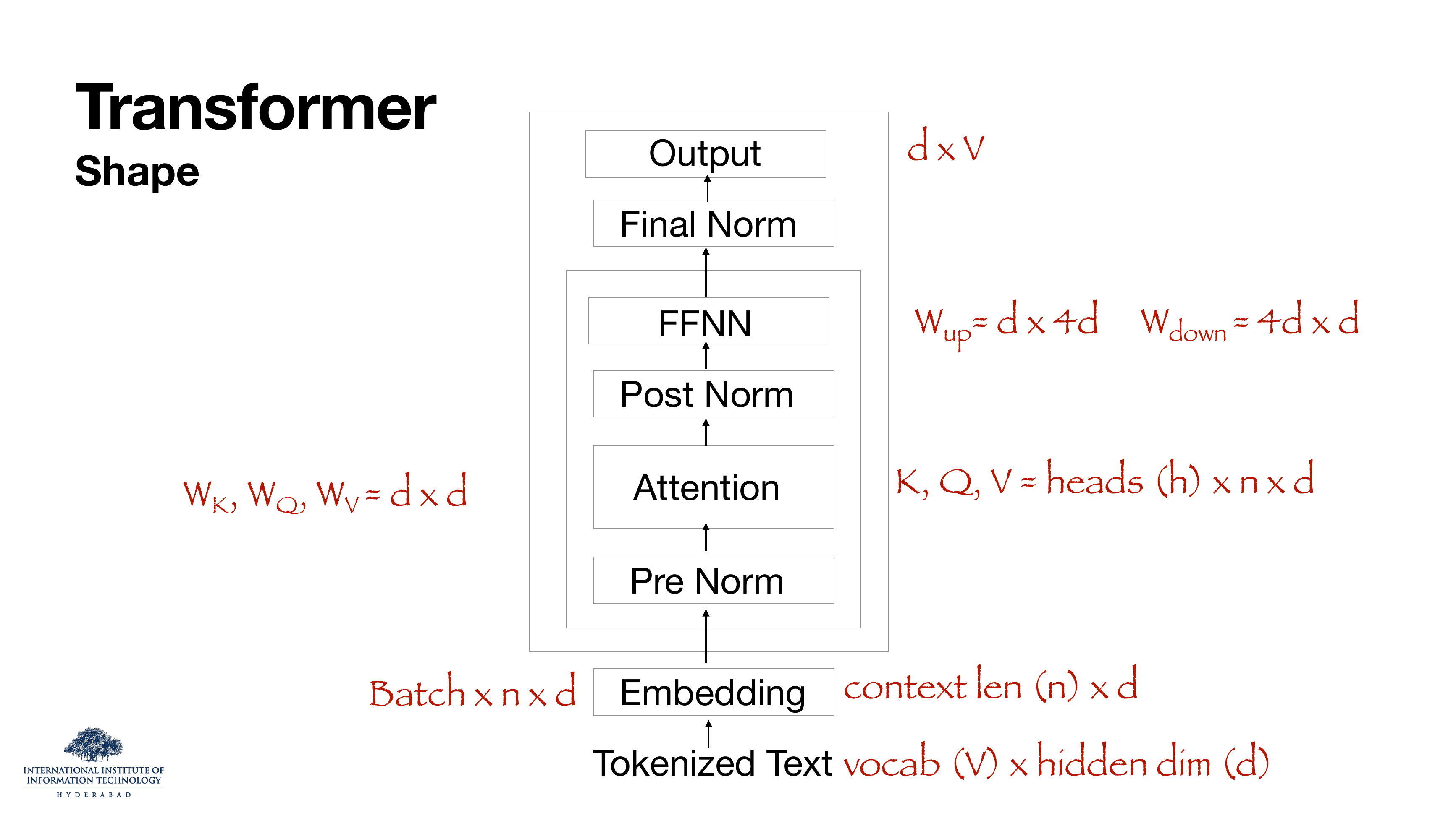
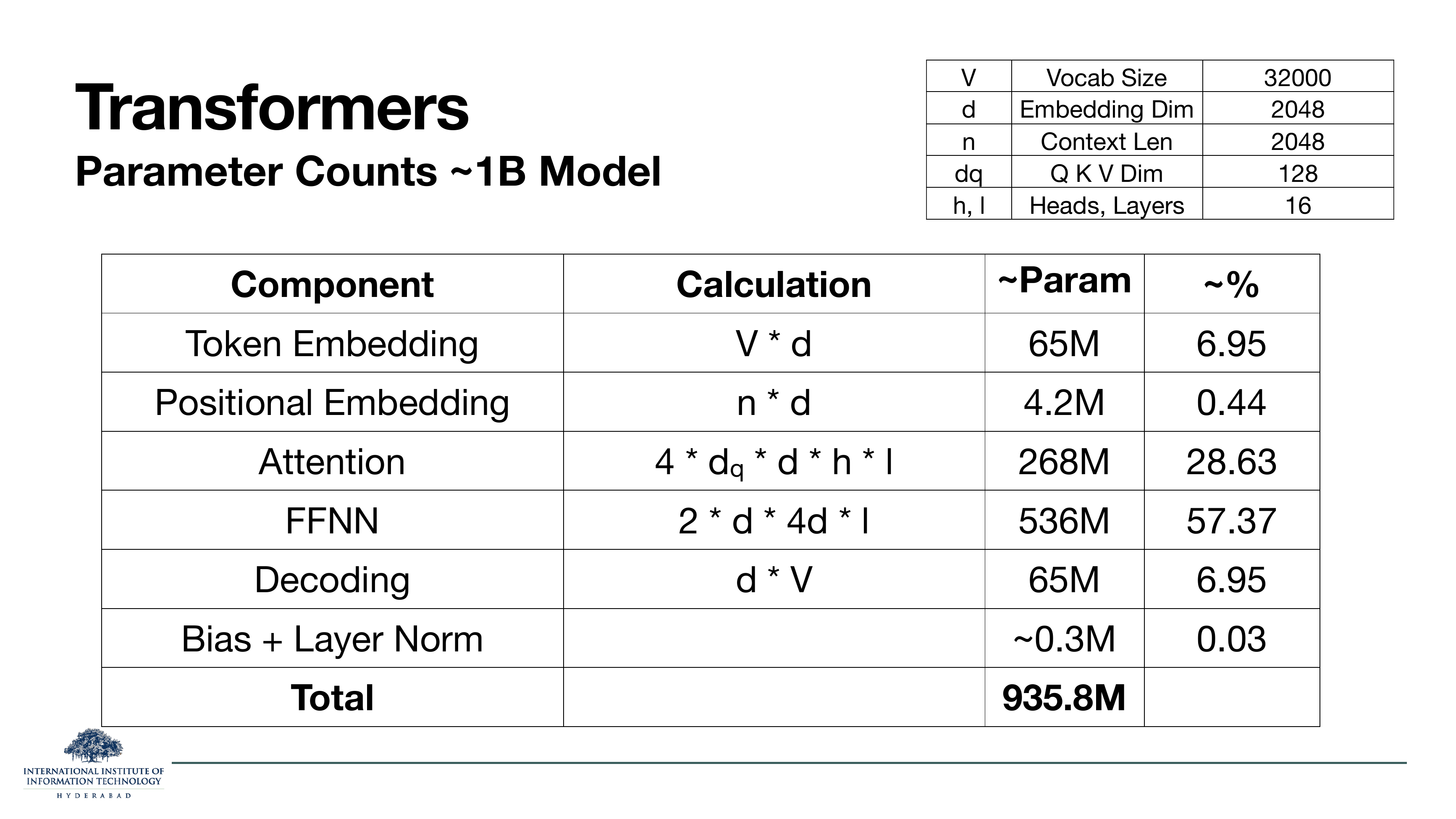
Slide 83 is a bookkeeping picture: given hidden dimension d, key dim d_q, h heads and vocabulary size V, every weight matrix has a specific shape. Slide 84 plugs in numbers (a 1B-parameter model with V=32k, d=2048, 16 layers, 16 heads) and reads off the budget.

✦ Key takeaway

Two numbers jump out. The FFN is 57% of the parameters. Attention (all four projections summed over all heads and layers) is 29%. Everything else is a rounding error. When people say "the transformer is mostly a stack of MLPs with a small amount of routing", this is what they mean.

Under the hood

You can also read the FFN's d×4d weight matrices as "one key-value memory per row". Two facts: (1) most of the model's factual knowledge sits in these matrices, (2) mixture-of-experts (MoE) works because you can shard them across experts without touching attention. Both are the "knowledge-stores" bullet on slide 79.

§10Where the field went next

Six slides. The lecture closes with a survey: how have transformer configurations drifted from 2017 to 2026, does "long context" actually work, and if it doesn't, where does it break? These slides do not teach a new mechanism; they orient you for the rest of the semester by naming names.

Slide 85 / 90

Transformer Models over Years table: Original Base (2017, 65M, 6 layers, sine PE, MHA, ReLU) through LLaMA/Mistral/LLaMA 3.2 (2023-24, RoPE + GQA + RMSNorm + SwiGLU) to DeepSeek V3, Qwen 3, Kimi K2 (2025, MoE, MHLA/GQA, up to 1T params).

slide 85 · nine years of drift

Slide 86 / 90

Transformer Models over Years 2026: Qwen 3.5, Sarvam, Nemotron 3 Ultra, Mistral 4, Gemma 4, Qwen 3.6, DeepSeek V4 (1.6T total / 49B active), Kimi K3 (2.8T / 104B). Announcement: Qwen 3.8 2.4T model announced.

slide 86 · the frontier, today

On these slides

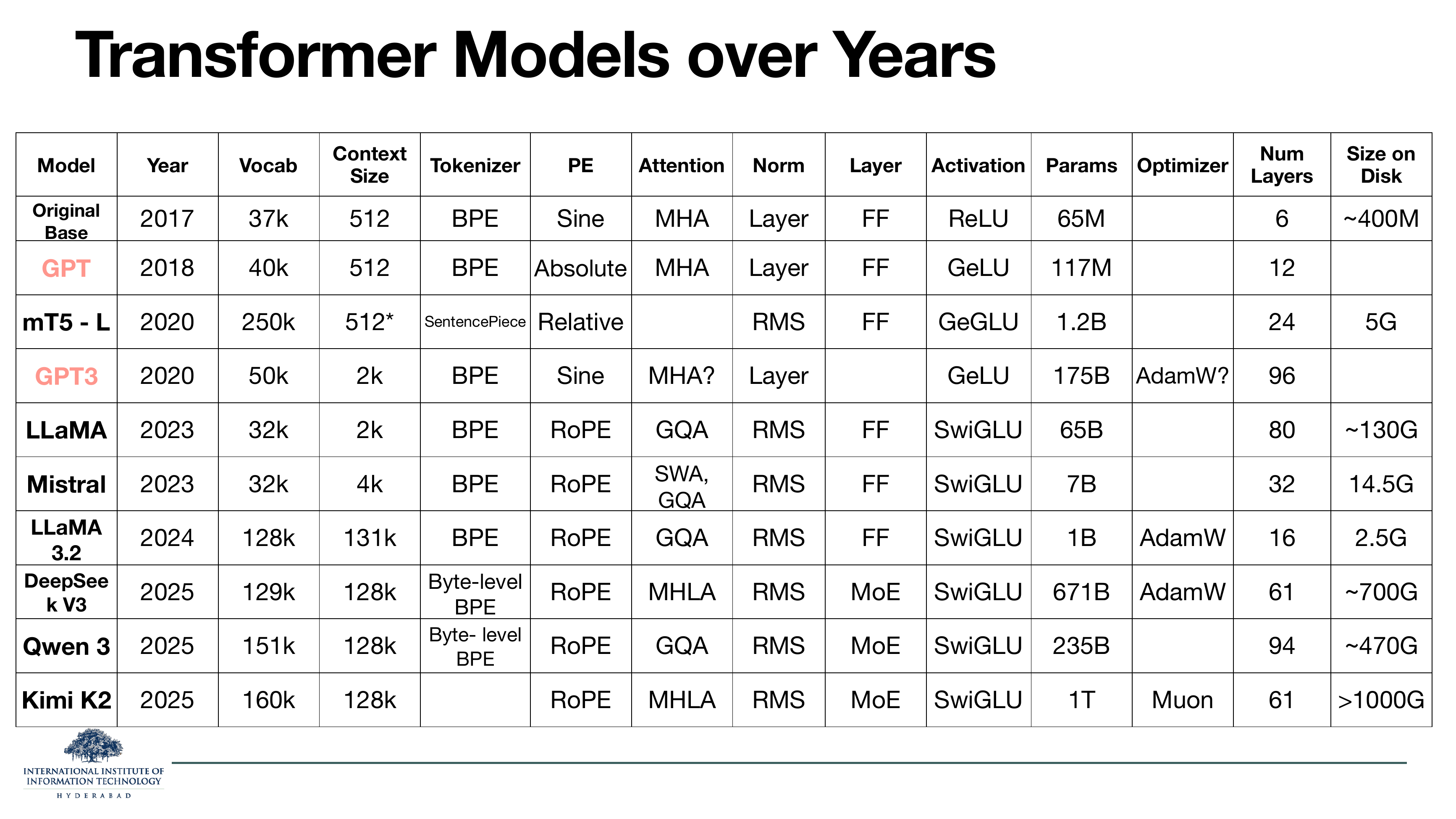
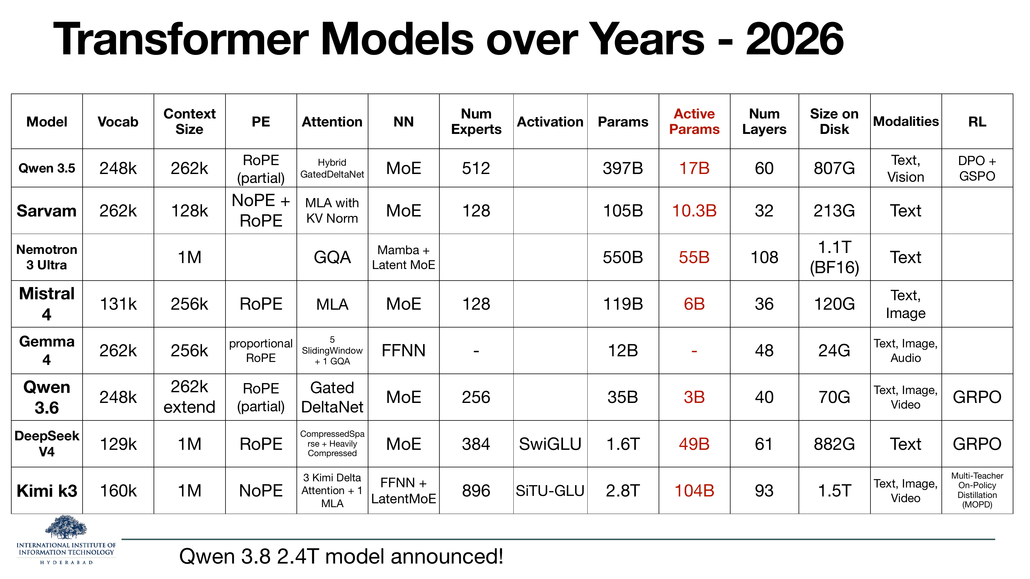
Two tables that map every headline model of the last nine years against the choices this deck has just introduced: tokenizer, positional encoding, attention variant, normalisation, activation, optimiser. Read them side by side and you can see the drift:

Positional encoding: sine → absolute → RoPE → NoPE.
Attention: MHA → GQA → MLA/MHLA (grouped or latent, both for KV-cache efficiency).
Normalisation: LayerNorm → RMSNorm (cheaper, no mean subtraction).
Activation: ReLU → GeLU → SwiGLU.
Layer type: plain FFN → Mixture of Experts (MoE) once you cross ~30B parameters.

✦ Key takeaway

Notice what has not changed: the block. It is still Add & Norm around attention, Add & Norm around a feed-forward, repeat N times. Every improvement in nine years is a swap-out of a single component, not a redesign. That is what "the architecture the field lives on" means.

→ Keep reading

Each column of these tables corresponds to one later lecture. Tokenizer → Lecture 3. PE → positional-encoding lecture. Attention → More Attention. Norm/Activation → the normalisation lecture. MoE → the MoE lecture. Come back to this slide at the end of the semester and every acronym will be a lecture you have taken.

Slide 87 / 90

Did we solve long contexts? Traditionally long contexts? Yes. Are there other long context tasks?

slide 87 · did we solve long context?

On the slide

A leading question. The 1M-token context lengths in slide 86 look like the long-context problem is solved. The lecturer is about to argue it is not. Classical benchmarks say yes, but the harder tasks say otherwise.

Slide 88 / 90

Large context inputs: documents (legal contracts, books, transcripts, reports), codebases, large system prompts to model.

slide 88 · what needs long context

Slide 89 / 90

Large context tasks: long-document question answering, multi-document QA/retrieval, long-history multi-turn conversations, code understanding.

slide 89 · what to do with it

On these slides

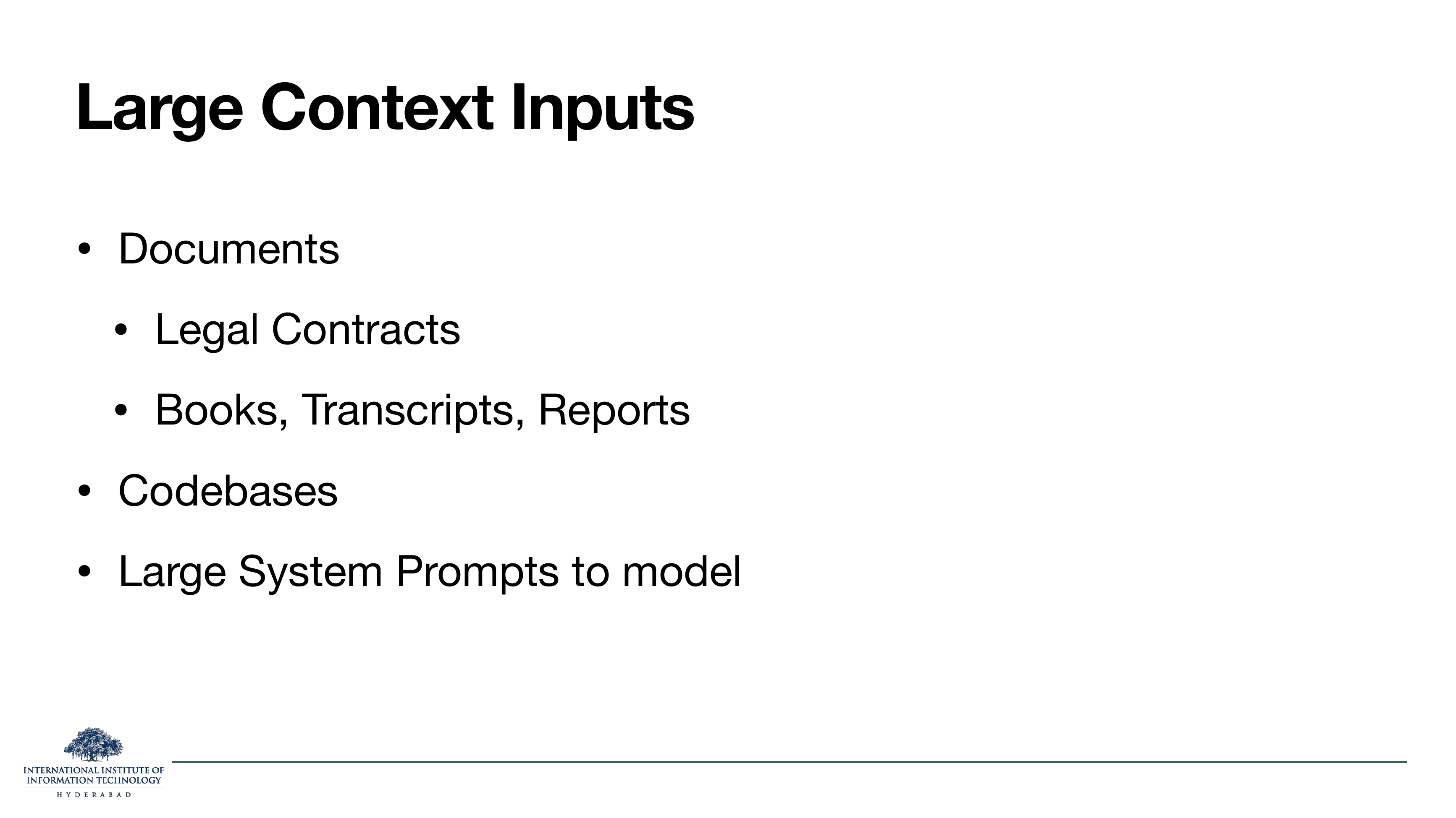
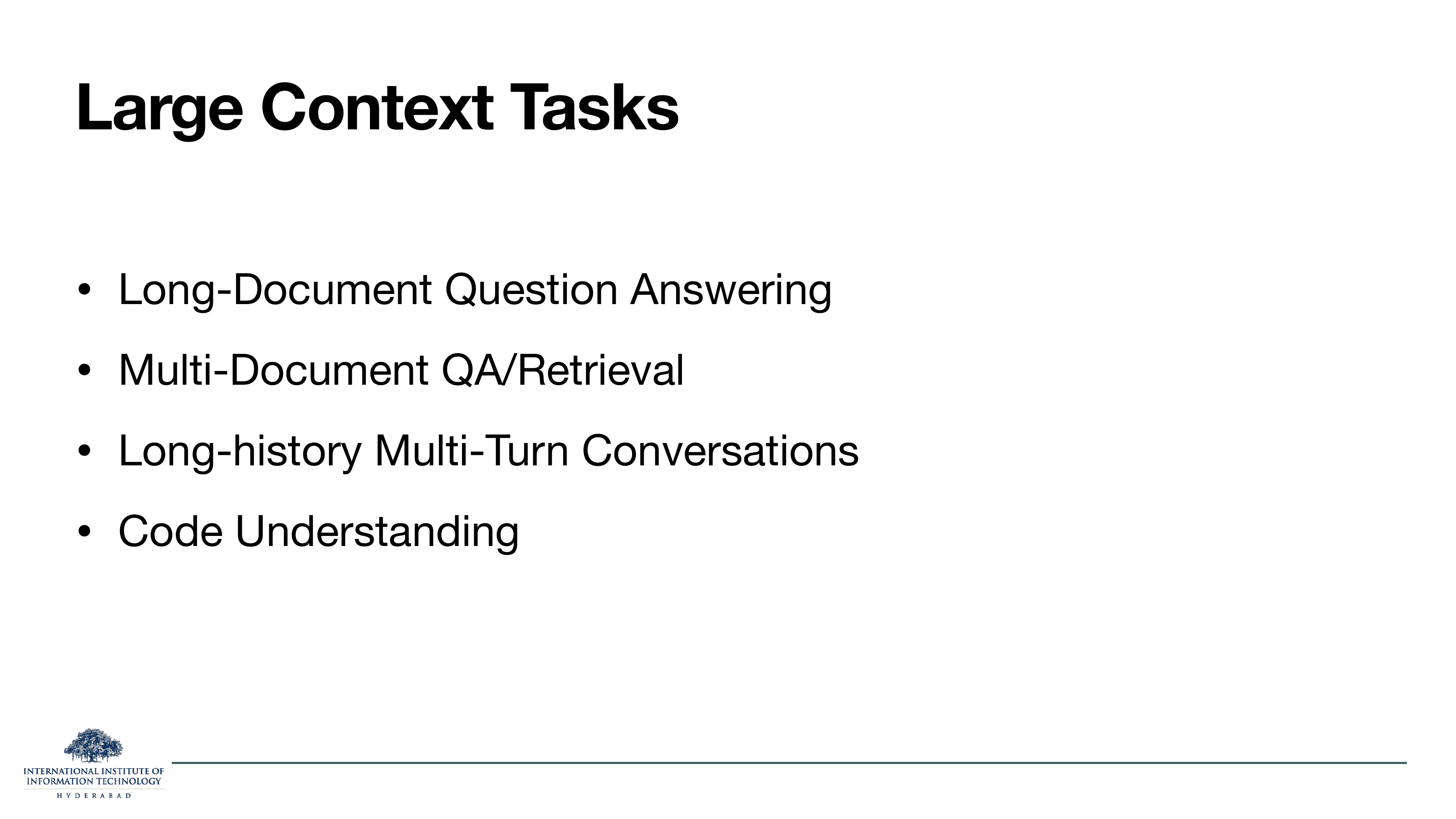
The real-world workloads that stress a model's context window. Inputs are legal contracts, whole books, transcripts, entire codebases, and multi-thousand-token system prompts. Tasks are long-document QA, multi-document QA / retrieval-augmented QA, long multi-turn dialogue history, and code understanding.

None of these are what the transformer was originally designed for. A machine-translation encoder eats a sentence, not a novel. Every one of them is where modern LLMs are asked to work today.

Slide 90 / 90

Lost in the Middle: model performance vs relevant information position — highest at beginning, high at end, significant degradation in the middle even for explicitly long-context models. Liu et al. 2024, TACL.

slide 90 · lost in the middle

On the slide

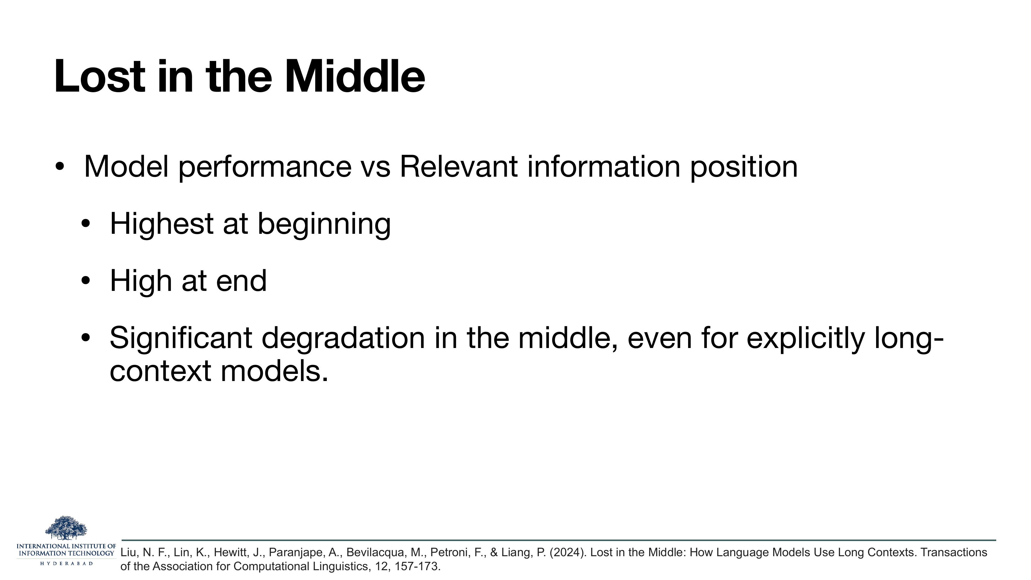
The closing punch. Liu et al. (TACL 2024) fed transformer LMs long documents with a single relevant fact hidden in them and measured accuracy as a function of where that fact sat. The curve is U-shaped: models find the fact well at the beginning, well at the end, and badly in the middle, even when the model's advertised context window comfortably fits the whole document.

⚠ the takeaway

A 128k-token context window is not the same as 128k tokens of attention. Positional encoding, attention dilution, and training-data recency all conspire to make the middle of a long input a blind spot. This one paper is why "long context" is still an open research area, not a solved engineering problem.

→ Keep reading

You will meet "Lost in the Middle" again in the retrieval / RAG discussion and in the long-context lecture. It is the reason many production systems chunk and re-rank rather than dump a whole document into context.

End of Lecture 2

Ninety slides in. You should now be able to (a) sketch the encoder-decoder transformer from memory, (b) name every arrow and say what problem it solves, and (c) read a modern LLM paper's architecture table and recognise every column. From here the course starts inside the block, piece by piece.