Mid Semester 2023 — the paper, worked through.
This is the 2023 mid-semester paper for M23CS7.501, with the instructor’s handwritten key. It has three conceptual questions worth 30 marks in 90 minutes. The notes below show the paper, decode the marking hints, and work through each answer clearly.
§1The paper
Q1 and Q2 are split into two five-mark parts. Q3 is worth 3 + 7, so the attention sub-question deserves most of your time. The paper is entirely about pre-transformer material.

Before you start
The paper is single-page and text-only. There are no diagrams to complete, no numeric problems, and no code. Every question is an open-ended "describe / explain / compare" prompt. This tells you two things about how the exam is graded.
- Marks are given for structure, not for showing intermediate arithmetic. A sub-part worth 5 marks expects roughly five distinct correct claims: a diagram, a defining equation, two mechanism sentences, and a "why".
- The 3 + 7 split on Q3 is the strongest signal on the paper. The 3-mark half is "describe seq2seq" (a diagram + one paragraph). The 7-mark half is "why attention". Spend your time there.
Because there is nothing to compute, students overwrite. A 5-mark answer that fills two pages of prose is not scoring more than a 5-mark answer that gives one diagram, one equation, and three tight sentences. The rubric caps at 5. Anything past that is time you owed to Q3.
§2The official key
The handwritten key is not a polished model answer. It is a compact list of the points the marker expected to see, which makes it useful for judging the level of detail each answer needs.
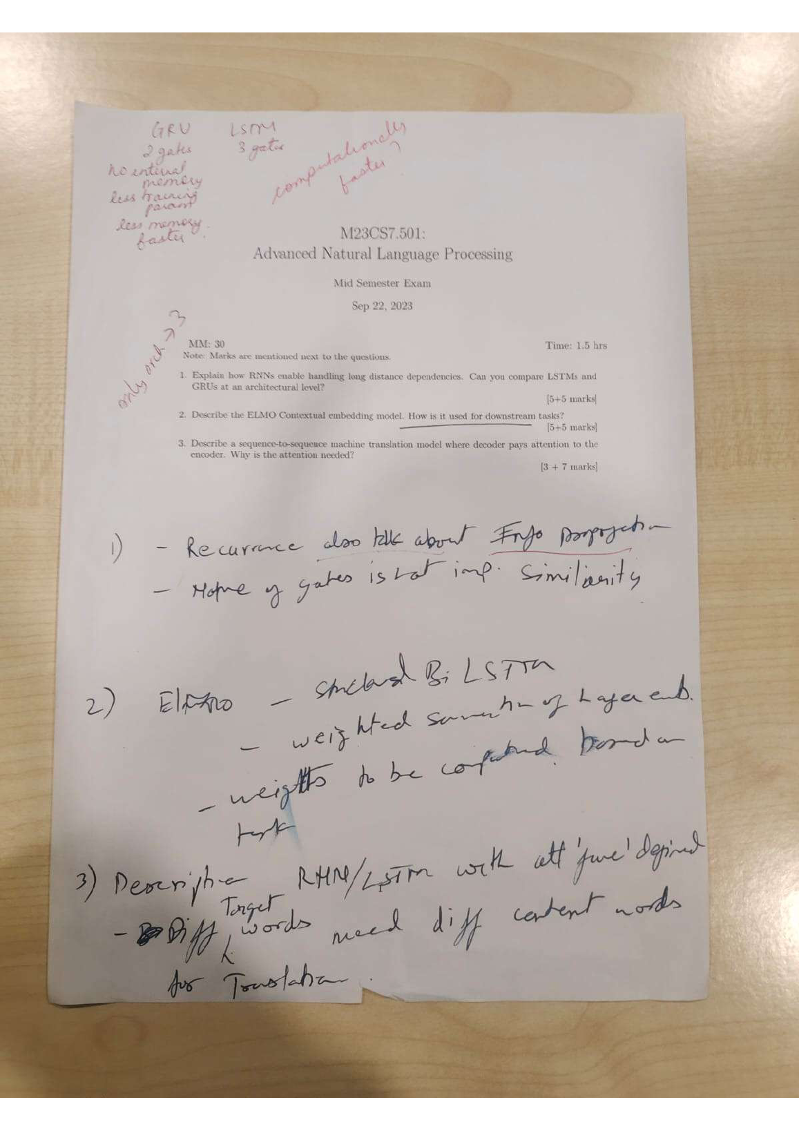
What the key says
Top margin (Q1 comparison table):
| GRU | LSTM |
|---|---|
| 2 gates | 3 gates |
| no external memory | computationally faster |
| less training params | |
| less memory · faster |
A vertical note in the left margin reads "only arch", a reminder that Q1 asks specifically for an architectural comparison, not a benchmark or an accuracy claim.
Q1: Recurrence — also talk about back propagation. Nature of gates is a lot important. Similarity.
Q2: ELMo — stacked Bi LSTM. Weighted summation of layer embeddings. Weights to be computed. Downstream task.
Q3: Describe a RNN/LSTM with attention "func" defined. Different target words need different content words for translation.
Each question's hint is roughly one bullet per mark. Q1 has four bullets (recurrence, backprop, gate nature, similarity) for five marks per sub-part. Q2 has four bullets (stacked BiLSTM, weighted sum, learn the weights, downstream). Q3 has two (define the attention function, argue different targets need different sources). Match that granularity in your own answer and you have a full-marks answer.
§3Q1 · RNN long dependencies, LSTM vs GRU
The question, verbatim
1. Explain how RNNs enable handling long distance dependencies. Can you compare LSTMs and GRUs at an architectural level? [5 + 5 marks]
How to approach it
The two sub-parts want different things. Sub-part (a) is a mechanism story: what does an RNN do that lets information from step 1 reach step 100. This means writing the recurrence, then honestly explaining the failure mode (vanishing gradients) and how gating is the general fix. Sub-part (b) is a side-by-side spec sheet: same structure of "here are the gates, here is the state, here are the equations", once for LSTM and once for GRU. The key's "only arch" note tells you to skip discussion of accuracy, dataset size, or training time; just architecture.
Worked answer
(a) How RNNs enable long-distance dependencies · 5 marks
A vanilla RNN reads a sequence , , …, one token at a time and maintains a hidden state that is recurrent: the state at step is a function of the previous state and the current input:
This is the mechanism that enables long-distance dependencies in principle. Because is a function of , and that of , the hidden state at time 100 has a functional path back to the input at time 1. Information about earlier tokens is carried forward through this shared recurrence, and the same weight matrices are reused at every step, so the model can learn a rule like "if a plural subject appeared, the verb far away must agree" without needing a separate parameter per gap length.
Training uses back-propagation through time (BPTT): the network is unrolled into a -layer feed-forward net that shares weights across layers, and the gradient of the loss with respect to flows backward through every previous step. Every backward step multiplies by the Jacobian , which is bounded by the spectral norm of times the derivative of .
This is where the vanishing / exploding gradient problem enters. If that Jacobian has spectral norm less than 1, gradients decay geometrically across steps and long-range signal never reaches the earlier weights; if greater than 1, they explode. So the architectural capacity for long dependencies (a recurrence) is real, but a plain RNN fails to train them in practice.
The fix that makes long dependencies actually learnable is gating. Instead of a single non-linear squash, a gated cell introduces sigmoid gates that decide, per component, how much of the old state to keep and how much of the new input to write. When a gate is near 1 on the "keep" path, the gradient flows across that time step nearly unchanged. This is the additive skip connection through time that gives LSTMs and GRUs their long-range memory.
Recurrence gives an RNN the capacity to carry information across time. Gates give it the trainability to do so, by turning the multiplicative gradient path into a nearly additive one on any step where the gate says "keep".
(b) LSTM vs GRU · architectural comparison · 5 marks
Both are gated RNN cells that replace the single update above with a small circuit of gates. They differ in how much state they carry and how many gates they use to route it.
LSTM. Keeps two state vectors: a cell state (long-term memory) and a hidden state (short-term / output). Three sigmoid gates control it: forget , input , output .
The forget gate erases parts of the old cell state; the input gate writes a candidate; the output gate decides what of the cell state becomes the exposed hidden state. The cell-state line is the constant error carousel: on any dimension where is near 1, the state passes through unchanged and gradients flow back undamped.
GRU. Collapses the cell state and hidden state into a single vector , and uses only two gates: update and reset .
The reset gate decides how much of the past to look at when computing the candidate. The update gate is a single interpolation knob between "keep the old state" and "replace with the new candidate", so it plays the role of the LSTM's forget and input gates fused into one. There is no separate output gate; the hidden state is exposed directly.
The side-by-side
| LSTM | GRU | |
|---|---|---|
| State vectors | and | only |
| Gates | 3 · forget, input, output | 2 · update, reset |
| How "keep" is expressed | independent and | tied via and |
| Exposed state | gated: | same as internal |
| Parameter count (hidden size ) | ≈ 4 · () · | ≈ 3 · () · |
| Constant-error path | through when ≈1 | through when ≈0 |
Similarities. Both are gated recurrences, both use sigmoid gates and a candidate, both preserve gradient flow through an additive path over time, and in practice both achieve comparable accuracy on most language tasks.
GRU is often preferred not because it beats LSTM on quality (it usually ties) but because it has roughly 25% fewer parameters and no separate cell state to store. Less memory, less compute per step, and one fewer gate to overfit. The LSTM's extra expressivity (independent forget and input, plus an output-gated view of the memory) pays off mainly on very long sequences and on tasks where the memory and the output need to look different.
What the key says
The key's four bullets (recurrence, backprop, nature of gates, similarity) line up with the solution above. The top-margin table (GRU 2 gates / no external memory / less params / less memory / faster vs LSTM 3 gates / computationally faster) is the marker's rubric for the comparison sub-part, and the side-by-side above hits every one of those rows. The vertical "only arch" reminder is the trap: do not lose time discussing which one wins on which dataset. The question is architectural only.
§4Q2 · ELMo and downstream use
The question, verbatim
2. Describe the ELMO Contextual embedding model. How is it used for downstream tasks? [5 + 5 marks]
How to approach it
Sub-part (a) wants the architecture: a stacked bidirectional LSTM language model, trained on a next-token prediction objective in both directions, whose per-layer hidden states become word representations. Sub-part (b) wants the recipe: one embedding per token is a learned weighted sum of the layer states, where the weights are task-specific parameters that are trained together with a downstream head while the ELMo LM itself is frozen. The key's four bullets are exactly this: stacked BiLSTM, weighted sum of layer embeddings, weights are trained, plug into downstream task.
Worked answer
(a) What ELMo is · 5 marks
ELMo (Embeddings from Language Models, Peters et al. 2018) is a contextual word-representation model: unlike GloVe or word2vec, the vector it assigns to the word bank depends on the sentence it appears in. The vector for bank in "river bank" differs from the vector for bank in "savings bank".
Architecturally, it is a stacked bidirectional LSTM language model trained on a large monolingual corpus:
- A character-CNN encodes each input token into a fixed vector . This makes ELMo robust to out-of-vocabulary words, so it can embed any string.
- A forward LM is a stack of LSTM layers (typically ) trained to predict from .
- A backward LM of the same shape is trained to predict from the right context.
- The two directions are trained jointly, maximising the sum of the forward and backward log-likelihoods.
After training, for a token at position the model produces representations: the token embedding , plus, at every layer , the concatenation of the forward and backward hidden states:
These per-layer vectors are the raw output of ELMo. The empirical observation Peters et al. make is that different layers capture different linguistic information: the lower layer is closer to syntax (POS, morphology), the higher layer is closer to semantics (word sense, coreference). That is why the final embedding is not just the top layer but a mixture across layers.
Bidirectional gives context from both sides. Without it, the vector for bank in "the bank of the river" would depend only on the words before bank. Stacked lets syntax and semantics live at different depths of the same tower, so the downstream model can choose which depth to lean on.
(b) How it is used for downstream tasks · 5 marks
For a downstream task, say NER or sentiment, ELMo is not fine-tuned. It is used as a frozen feature extractor. For each token, the task model receives one vector produced by taking a learned weighted sum of the ELMo layers, scaled by a per-task gamma:
Here are softmax-normalised layer weights (they sum to 1) and is a scalar that scales the mixed vector to a magnitude the downstream head is comfortable with. Both are learned during downstream training; they are the only ELMo-side parameters the task ever updates.
The full recipe:
- Take the pre-trained ELMo LM and freeze it.
- Run the input sentence through it once to get for every token and every layer.
- Compute with the current learned and .
- Concatenate that vector with a static input embedding (GloVe / word2vec) if one is used, giving .
- Feed that concatenated vector into the task-specific model (a BiLSTM for NER, a classifier for sentiment, an encoder for QA) and train that model end-to-end. Gradients flow back into , , and the task model, not into the ELMo LSTMs.
Optionally, ELMo can also be inserted at the output side of the task model instead of the input, and the paper shows that using it at both ends helps some tasks.
The learned is what makes ELMo more than "just the top layer of a BiLSTM". A syntactic task (POS tagging) will learn to lean on the lower LSTM layer; a semantic task (word sense disambiguation) will learn to lean on the upper one. One frozen encoder can serve every downstream task because each task picks its own mixture.
What the key says
The key's four bullets (stacked Bi LSTM, weighted summation of layer embeddings, weights to be computed, downstream task) are exactly the four things above. "Weights to be computed" specifically means the and are learned, not fixed. A common mistake is to describe ELMo as "just concatenate all the layers" or "just take the top layer", both of which drop that mark.
§5Q3 · Seq2seq with attention
The question, verbatim
3. Describe a sequence-to-sequence machine translation model where decoder pays attention to the encoder. Why is the attention needed? [3 + 7 marks]
How to approach it
The mark split is the most important thing on this question. The 3-mark half is describing an encoder-decoder RNN with attention: a diagram plus one paragraph is enough. The 7-mark half is why attention is needed. Do not answer this with a single sentence. The full argument has three moves: the bottleneck problem in vanilla seq2seq, the "different target words need different source content" observation from the key, and the concrete alignment computation that solves it.
Worked answer
(a) The model · 3 marks
A sequence-to-sequence machine translation model with attention has three pieces:
- An encoder BiLSTM reads the source sentence and produces one hidden state per source position, . These are the encoder annotations.
- A decoder LSTM generates the target sentence one token at a time. At target step , its hidden state is .
- An attention block sits between the encoder and the decoder. At every decoder step, it looks over all encoder annotations and produces a context vector : a weighted sum of the encoder states, where the weights are computed from how well each source state matches the current decoder state.
The decoder then produces the next target token from its own state and this context vector: .
(b) The attention function · part of 7 marks
At decoder step , attention runs three lines:
The score function is the "attention func" the key wants defined. Two standard choices:
Additive (Bahdanau, 2015). A tiny feed-forward net:
Multiplicative / dot (Luong, 2015). Cheaper: just a dot product, optionally with a learned matrix in the middle:
Once is computed, the decoder uses both its own state and the context to predict the next word. In Bahdanau's formulation the context is fed into the decoder RNN update; in Luong's it is concatenated with the decoder state after the update. Either way, the decoder step becomes conditioned on a source view that changes at every target position.
(c) Why attention is needed · the rest of 7 marks
The bottleneck problem. A vanilla seq2seq encoder-decoder (Sutskever et al. 2014) reads the whole source sentence and summarises it into a single fixed-length vector (the final encoder hidden state) and hands that one vector to the decoder as its only source-side input. The decoder must generate the entire target sentence from this single vector. Empirically this collapses on long sentences: translation quality drops sharply once the source is longer than roughly 20 to 30 tokens, because a fixed-size vector cannot carry all of the source content.
Different targets need different source content. This is the key's core observation. Consider translating "the red car is fast" into French, "la voiture rouge est rapide". When the decoder is producing voiture, it needs to look at car. When it is producing rouge, it needs to look at red. A single fixed source vector cannot serve both; it either averages the two signals or forgets one. What the decoder actually needs is a different source view at each target step. That is exactly what attention gives: a fresh per step, computed by softly pointing at the source tokens that matter for the current output.
Attention lifts the bottleneck by letting the decoder look back. The encoder no longer has to fit the whole source into one vector, because every one of its per-position states is preserved and reachable. At each decoder step, the softmax over alignment scores acts as a soft pointer: it selects (or blends) the source positions relevant to what the decoder is about to output. In effect, the decoder can "look back" at any encoder state at any time, cost-free at inference.
The alignment side-effect. The attention weights also give a free, interpretable soft alignment between source and target words, which was previously a separate step in phrase-based statistical MT systems. Attention absorbs alignment into the model.
Vanilla seq2seq forces one source vector to serve every target step. Attention gives every target step its own source vector, computed by a soft, differentiable lookup over the encoder's per-position states.
Attention is more than an accuracy fix for long sentences. It is the observation that "which piece of the input do I need right now" is itself something the model can learn. Once you can learn a soft lookup over encoder states, you no longer need recurrence to carry information across positions; you can just attend directly. That realisation is what leads, three years later, to the transformer.
What the key says
The key's two bullets are (i) describe a RNN/LSTM with attention "func" defined, hit in the alignment score above, and (ii) different target words need different content words for translation, hit in the "why" argument. The mark split (3 + 7) is worth remembering next year: describing the model is cheap, defending attention is where the marks live.