Talking Matrices: from embeddings to BERT.

On the slide

The title slide. Talking Matrices: And other prerequisites, delivered on 8 August 2026 at IIIT Hyderabad.

What it means

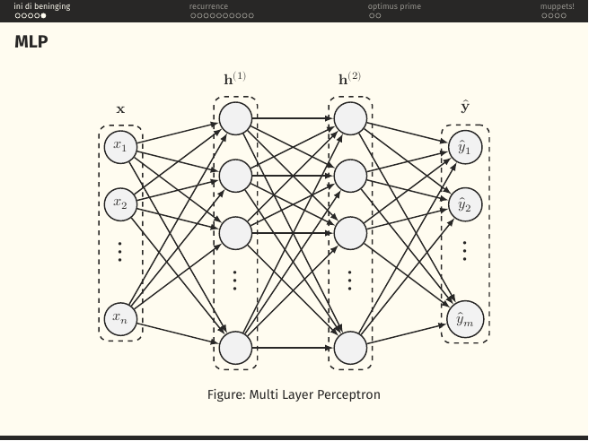
The joke in the title is that all the neural machinery you will meet in this course is, at heart, matrices talking to matrices. A word becomes a row of numbers, a sentence becomes a stack of rows, a network is a chain of matrix multiplies with a nonlinearity between each pair, and training is the slow rearrangement of those numbers by gradient descent. Everything else, the diagrams, the exotic cell drawings, the muppet mascots, is just naming schemes over that same operation.

A section divider. Everything until page 06 is about the pre-deep-learning question: how do you turn a word into a vector at all?

On the slide

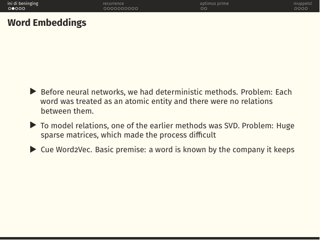
A three-beat history of word representation. Before neural nets, words were atoms, one-hot vectors with no notion of similarity between "king" and "queen". People tried to fix this with count-based statistics and SVD on a co-occurrence matrix, which worked in principle but produced enormous, mostly-zero matrices. Then Word2Vec (Mikolov, 2013) reframed the problem: learn a dense vector for each word by predicting its context.

What it means

The Firthian slogan on the last bullet, "a word is known by the company it keeps", is the entire justification for distributional semantics. If two words show up in the same neighbourhoods (doctor, nurse) their meanings are close; if they never co-occur (doctor, banana) they are not. Every embedding technique from Word2Vec through GloVe to BERT's contextual embeddings is a refinement of this one bet.

On the slide

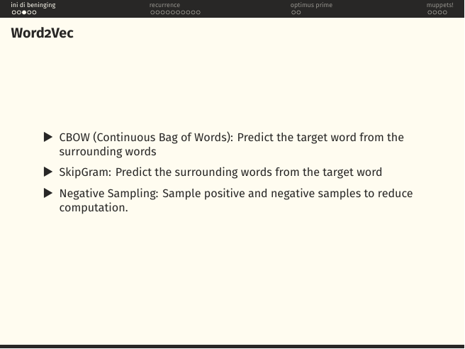
The three ingredients that make Word2Vec work: two training objectives and one computational trick.

• CBOW (Continuous Bag of Words): given the context words in a small window, predict the missing centre word. Averages the context embeddings and asks a softmax to name the target.
• SkipGram: flip it. Given the centre word, predict each context word independently. Empirically better for rare words because every occurrence teaches the model something.
• Negative sampling: the honest softmax over a 100K-word vocabulary is unaffordable. Replace it with a binary classifier, is this a real (word, context) pair or a randomly sampled fake one?, and you only touch a handful of vectors per update.

What it means

Notice what Word2Vec is not: it is not a deep network. It is a shallow, essentially linear model whose only nonlinearity is the sigmoid on the final classifier. The magic is not in depth; it is in the objective. You train on billions of context windows and the geometry of the resulting embedding space starts to encode analogies, the famous $\mathrm{king}-\mathrm{man}+\mathrm{woman}\approx \mathrm{queen}$.

On the slide

A section divider and then the diagram everyone draws when they say "neural network": an input $x$, two fully-connected hidden layers $h^1$ and $h^2$, and an output $\hat{y}$. Every arrow is a weight; every circle applies a nonlinearity to the sum of its inputs.

What it means

An MLP is a stack of affine transforms interleaved with nonlinearities. In matrix form:

$h^1=\sigma (W_{1}x+b_1)$
$h^2=\sigma (W_2{h}^1+b_2)$
$\hat{y}=\mathrm{softmax}(W_3{h}^2+b_3)$

That is the whole engine. A universal function approximator in principle. But look what it lacks: nothing in this picture cares that the input is a sequence. Feed it "the cat sat" and "sat cat the" as bags of one-hots and it will happily produce the same output. That defect is the reason the next section exists.

A section divider. The next ten pages are the recurrent story.

On the slide

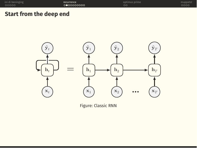
The founding picture of the RNN. On the left, a single cell with a loop from its hidden state back to itself. On the right, that same cell drawn out across time, $h_1,h_2,\dots ,h_T$, with each step taking a new input $x_t$ and emitting a prediction ${\hat{y}}_t$.

What it means

The RNN's whole contribution is one word: share. Instead of an MLP with a separate weight matrix for each timestep, you have one matrix that gets applied over and over. Whatever the network learns about how to update its memory when it sees a verb at step 3, it also uses at step 47. That parameter sharing is what makes learning from sequences tractable at all.

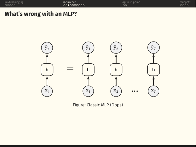
On the slide

The same picture as page 08 with one detail changed: the horizontal arrows between hidden states are gone. Now it is just a stack of independent MLPs, one per timestep.

What it means

This is what an MLP would do if you naively applied it word-by-word. Each step processes its input in isolation. Nothing carries forward. Feed it "not bad" and the "bad" step has no idea it was just negated. This is the context problem, and the horizontal arrow of the previous slide, the recurrence, is the whole answer.

On the slide

The vanilla RNN cell, opened up. The previous hidden state $h_{t-1}$ and the current input $x_t$ are concatenated, pushed through a single learned linear layer, and squashed by a $\tanh$. The result is both the new hidden state $h_t$ and (after one more projection) the output ${\hat{y}}_t$.

What it means

The compact form is:

$h_t=\tanh \left(W\right[x_t;h_{t-1}\left]\right)$

Note what "concatenate then multiply by $W$" secretly is: $W_x{x}_t+W_h{h}_{t-1}$. Two matrices masquerading as one. Everyone writes it the concatenated way because it looks tidier on a slide.

On the slide

The Long Short-Term Memory cell (Hochreiter & Schmidhuber, 1997), a vanilla RNN's better-behaved cousin. It carries two states, not one: an internal cell state $c_t$ that runs along the top of the diagram like a conveyor belt, and the usual hidden state $h_t$. Three sigmoid gates decide what to do with the belt:

• Forget gate $f_t$, multiplies the old cell state elementwise. Zero means forget, one means keep.
• Input gate $i_t$, decides how much of the new candidate ${\tilde{c}}_t$ to add.
• Output gate $o_t$, decides how much of the (tanh'd) cell state to expose as the new hidden state.

What it means

The magic is the top wire: the cell state passes through only additive updates and elementwise multiplications by a sigmoid. There is no repeated matrix multiply on that path. So when you backpropagate along the belt, gradients survive across dozens of timesteps rather than vanishing after five. That, and nothing else, is why LSTMs beat vanilla RNNs on real sequence tasks for two decades.

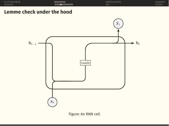
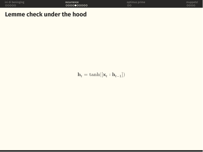
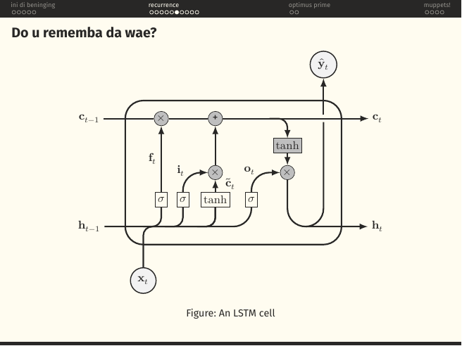
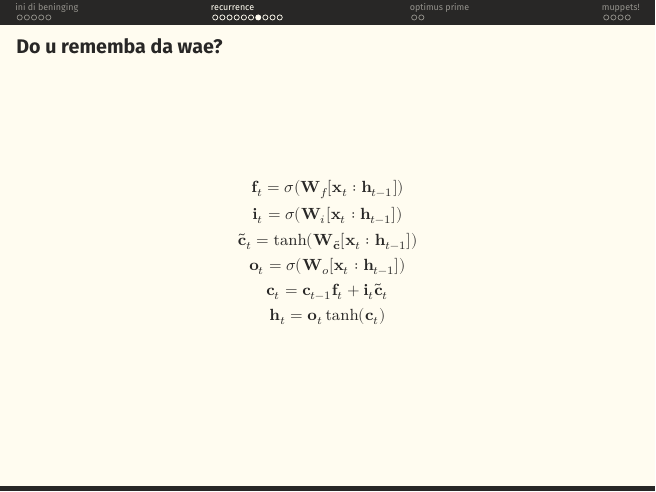
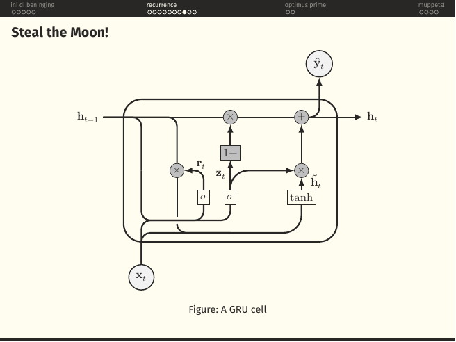
On the slide

The Gated Recurrent Unit (Cho et al., 2014), the LSTM stripped down. Two gates instead of three, and no separate cell state at all, the hidden state doubles as the memory.

• Reset gate $r_t$, decides how much of the old hidden state feeds into the candidate.
• Update gate $z_t$, a single knob that interpolates between "keep old" and "take new". The diagram's $1-$ block is what makes this a convex mixture.

What it means

Formally: $h_t=(1-z_t)\odot h_{t-1}+z_t\odot {\tilde{h}}_t$. Fewer parameters than an LSTM, comparable performance on most tasks, faster to train. The empirical answer to "do we really need three separate gates?" turned out to be: often, no.

On the slide

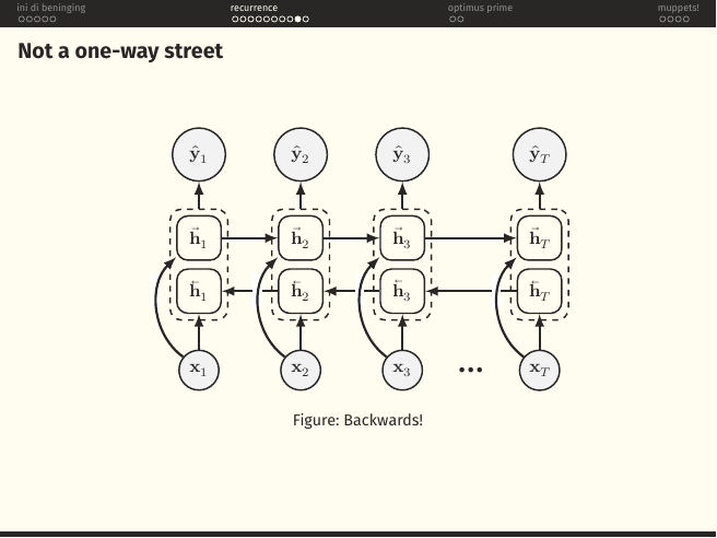
A bidirectional RNN. Two independent recurrent passes over the same input: one left-to-right (${\overrightarrow{h}}_t$) and one right-to-left (${\overleftarrow{h}}_t$). At each timestep the two are concatenated before predicting ${\hat{y}}_t$.

What it means

A unidirectional RNN's hidden state at step $t$ knows about the past but not the future. That is fine when you are generating, one token at a time. It is a real limitation when you are tagging, labelling every word in a sentence, because "bank" in "river bank" needs the word "river" to disambiguate, and "river" comes after in some dialects of the same idea. The bidirectional variant fixes this at the cost of doubling the compute and forbidding streaming inference.

On the slide

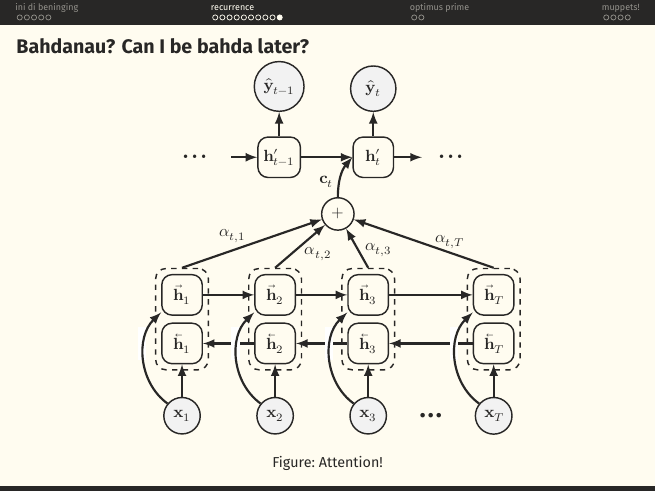
The single most important slide in this section. Bahdanau, Cho and Bengio's 2015 attention mechanism, drawn over an encoder-decoder architecture. The encoder is a BiRNN. The decoder, at each step $t$, does not receive a single fixed context vector; it receives a weighted sum $c_t=\sum _i{\alpha }_{t,i}{h}_i$ of the encoder hidden states, where the weights ${\alpha }_{t,i}$ are computed on the fly.

What it means

Before Bahdanau, the entire source sentence in a neural translation model was squeezed into one fixed-size vector. Long sentences failed because you cannot cram a paragraph into 512 floats without loss. Attention broke the bottleneck: at every decoder step, the model gets to look at the encoder states directly and decide which ones matter for the word it is about to emit. The weights $\alpha$ are a soft version of "which source word am I translating right now".

A section divider. The recurrence is gone; attention is the whole engine now.

On the slide

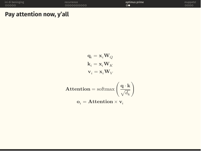
The attention operation in six lines. Each input vector $x_i$ is projected three ways into a query $q_i$, a key $k_i$ and a value $v_i$ by three learned matrices $W_Q,W_K,W_V$. The attention weights are:

$\mathrm{Attention}=\mathrm{softmax}\left(\frac{q·k}{\sqrt{d_k}}\right)$

And the output at position $i$ is the corresponding weighted sum of value vectors.

What it means

The database metaphor is exact: every position gets to query every other position, matches its query against those positions' keys, and pulls back a soft-lookup of the corresponding values. The $\sqrt{d_k}$ in the denominator is not decorative: without it, at large $d_k$ the dot products grow, the softmax saturates, gradients vanish, and training stalls. Vaswani et al. discovered this scaling empirically and it is now folklore.

A section divider. From this page on, "embedding model" means contextual embedding: the vector for a word depends on the sentence it sits in.

On the slide

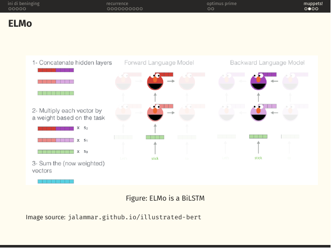
ELMo (Embeddings from Language Models, Peters et al. 2018) built on top of a two-layer bidirectional LSTM language model. For any word in a sentence, it stacks the forward and backward LSTM hidden states at every layer, weighs them by task-learned scalars $s_0,s_1,s_2$, and sums the result into one contextual vector.

What it means

Word2Vec gave you one vector per word, forever. ELMo gave you a different vector for "bank" depending on whether it appeared next to "river" or next to "loan". That single shift, from a lookup table to a function of the sentence, is what made the muppet era possible.

On the slide

Two views of the same object. First, BERT as a friendly yellow blob: 512 tokens go in, 512 contextual vectors come out. Then, the blob opened up to reveal 12 identical transformer encoder blocks stacked on top of each other. (BERT-large uses 24.)

What it means

BERT (Devlin et al., 2018) is what you get when you take the transformer encoder from section §3, throw away the decoder entirely, and pretrain the encoder on two self-supervised objectives on a mountain of text:

• Masked Language Modelling. Randomly hide 15% of the input tokens and ask the encoder to guess them back. Because attention is bidirectional inside an encoder, the model gets to look both left and right, the muppet update of ELMo's core trick.
• Next Sentence Prediction. Given two segments, decide whether the second one follows the first. Later work (RoBERTa) showed this objective barely helps; the MLM does most of the heavy lifting.

Once pretraining is done, you attach a tiny task-specific head to the $\left[\mathrm{CLS}\right]$ vector (for classification) or to the per-token outputs (for tagging) and fine-tune. That is the whole recipe.

On the slide

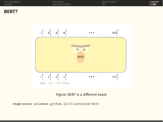
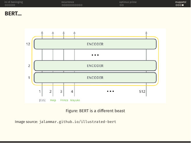
The end card. Fin. From atomic one-hot vectors to a stack of twelve transformer encoder blocks, in twenty-two slides.

What it means

If you sat with every page here you now have the whole ladder in view: Word2Vec teaches you that words can live in a geometry; the MLP teaches you what a learned function looks like; the RNN teaches you why sequence order matters and why plain backprop through time is a nightmare; LSTM/GRU teach you the additive-path trick that saves gradients; attention teaches you that you can just look instead of remember; the transformer removes the crutch of recurrence entirely; and BERT shows that once you have a good encoder, all of NLP starts to look like fine-tuning one big pretrained model. The rest of this course is what happened next.