Tutorial 01 · 82 pages · August 7, 2026

Mathematics for Deep Learning: and other abstract nonsense.

Before the transformer, before attention, before any of the machinery the rest of the course spends the semester on, there is a very small pile of math you cannot get away with not knowing. This tutorial is that pile. It walks from what a vector is to why the last layer of a language model is a softmax, and it does so in eighty-two deliberately slow pages. Read it once now. Come back to it whenever a later slide has a matrix in it and you find yourself squinting.

Tutorial 01 82 pages math prerequisites

§0The tutorial at a glance

The deck is organised into four sweeps, tracked by the four dot-rows along the top of every page. Early days is a one-slide confession about prerequisites. Linear algebra takes you from vectors to LoRA in eight pages. Calculus spends the most time in the room, because every hard idea in deep learning is either a derivative or an update built from one, partials, gradients, Jacobians, Hessians, gradient descent, Newton-Raphson, and a hint of the SVD trick that powers modern optimisers. Finally Deep learning assembles all of the above into a parametrised function, argues from the Universal Approximation Theorem that it is enough, then walks the chain rule back through the layers to build backpropagation, SGD, Adam, and eventually softmax over a vocabulary. That last step is where NLP starts.

§1Early days

Two pages of ground-clearing. A cover slide, and a very honest prerequisites list.

Page 01 / 82

$Title slide: Mathematics for Deep Learning — And other abstract nonsense, aNLP M'26, August 7 2026, IIIT Hyderabad.$

page 01 · title

On the slide

Mathematics for Deep Learning: And other abstract nonsense. A tutorial slot, not a lecture, delivered on August 7, 2026, one week into the semester.

What it means

The subtitle is doing a lot of work. "Abstract nonsense" is a fond mathematician's phrase for category-theoretic hand-waving, the kind of reasoning that pushes symbols around at a level so general that it forgets what it started with. The joke is that deep learning does exactly this: it takes clean linear-algebra objects, stacks them, differentiates them with respect to millions of parameters, and shrugs when the resulting update doesn't quite make geometric sense. The tutorial's promise is to keep the abstract nonsense down to a working amount.

Page 02 / 82

$Prereqs page: basic linear algebra (idea of a vector and a matrix), basic calculus (derivatives), or barebones intuition — alternatively, a 3Blue1Brown subscription.$

page 02 · """"prereqs""""

On the slide

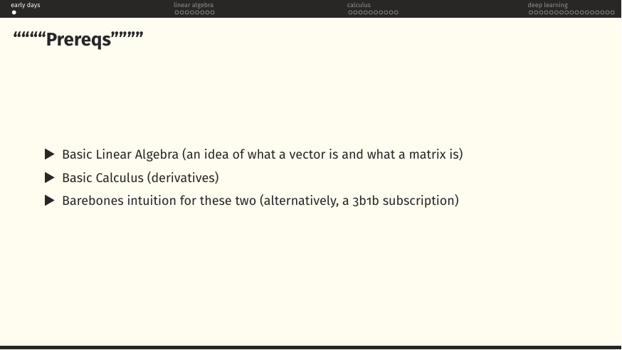
The quote-marks around "Prereqs" are load-bearing. The list is short: know what a vector is, know what a matrix is, know what a derivative is. Or, and this is the honest fallback, have watched enough 3Blue1Brown that you can picture those objects even if you cannot manipulate them yet.

◉ how to read this tutorial

Everything past page 3 assumes you can nod along at the sentence "a matrix is a function that eats a vector and returns another vector". If that sentence feels foreign, watch Essence of Linear Algebra chapter 3 before proceeding. If it feels obvious, skim quickly, the tutorial builds slowly on purpose.

§2Linear algebra: vectors to LoRA in eight pages

Eight pages. The route: definition of a vector space, matrices as maps between them, two families of "nice" matrices (diagonal and orthogonal), eigenvectors as invariant directions, and finally the outer-product / low-rank story that gives us LoRA. If the last page reads like a magic trick, that is the whole point of the six pages leading up to it.

Page 03 / 82

$Section divider: Linear Algebra Foundations.$

page 03 · section divider

A section divider. Everything from here to page 10 is linear algebra.

Page 04 / 82

$Vector spaces, bases, linear combinations, span.$

page 04 · vectors, spaces, bases

On the slide

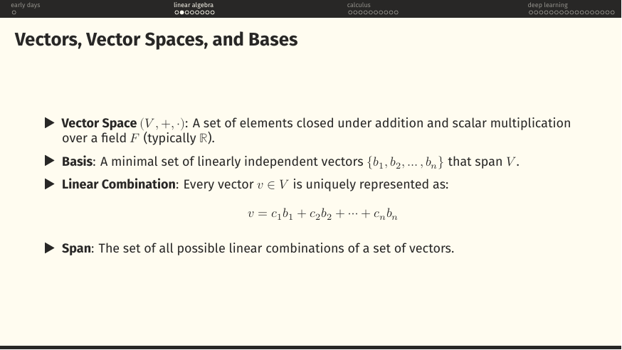
Four definitions stacked on top of each other: vector space, basis, linear combination, and span.

What it means

Forget the axioms for a second. A vector space is any collection of things you can add together and scale by numbers without leaving the collection. Arrows in the plane qualify. Polynomials of degree at most 5 qualify. So do functions from ℝ to ℝ. A basis is a smallest set of these things such that every other one is a unique recipe of "add this much of the first, then this much of the second". The recipe itself is called the linear combination; the set of all possible recipes is the span.

✦ the aha

The whole reason we get to talk about "coordinates", $v = (3, − 1, 4)$ , is that a basis exists. The numbers are the recipe. Change the basis, change the recipe, but not the underlying arrow.

Page 05 / 82

$Matrices as linear transformations. A ∈ ℝ^{m×n} defines T: ℝ^n → ℝ^m. Columns of A tell you where the standard basis vectors land.$

page 05 · matrices as maps

On the slide

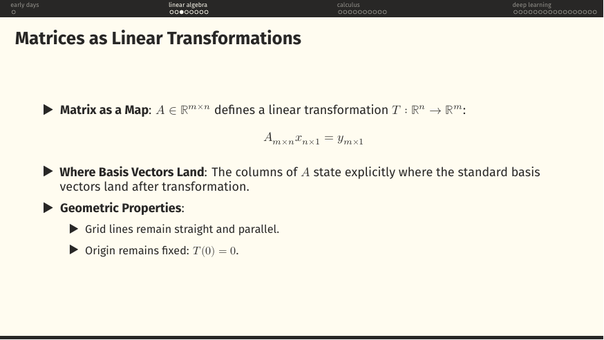
A matrix $A$ of shape $m \times n$ is not a number-grid, it is a linear transformation, a function that eats an $n$ -vector and hands you back an $m$ -vector.

What it means

The most useful thing to know about any matrix is this: its columns tell you where the standard basis vectors go. Column 1 is where $e = (1, 0, \dots)$ lands after the transformation, column 2 where $e 2$ lands, and so on. Everything else, matrix-vector product, matrix-matrix product, determinant, falls out of this one fact.

Two consequences of linearity worth internalising: grid lines stay straight and parallel after the transformation, and the origin never moves. If either fails, you are not looking at a linear map.

◉ mental model

When you see $y = A x$ , read it as "y is a linear combination of A's columns, weighted by the entries of x." Every matrix product you meet for the rest of the course is a version of this sentence.

Page 06 / 82

$Primitive spatial transformations: diagonal matrices scale along axes; orthogonal matrices Q^T Q = QQ^T = I are rotations or reflections and preserve lengths and angles.$

page 06 · diagonal & orthogonal

On the slide

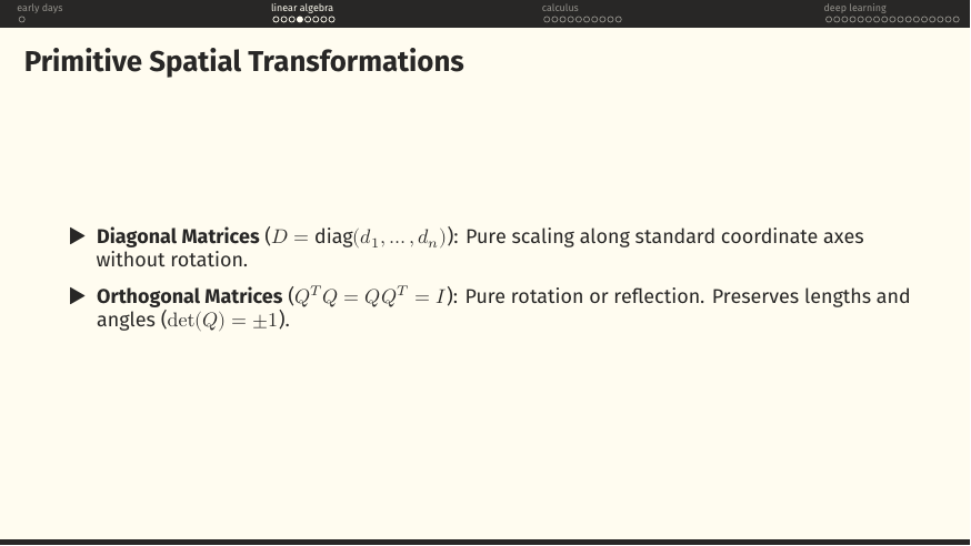
Two families of "clean" matrices: diagonal matrices, which stretch each axis independently, and orthogonal matrices, which rotate or reflect but preserve every length and every angle.

What it means

These are the atoms out of which every other linear transformation is built. The Singular Value Decomposition, which will haunt us later, says that any matrix, no matter how ugly, factors into rotate, then scale along the axes, then rotate again. That is $A = U Σ V^{T}$ . When we hit low-rank matrices in two pages, this is why the picture is so clean.

✦ the aha

$\det (Q) = \pm 1$ is not a formula, it is a geometric fact: orthogonal matrices preserve volume. Positive determinant means a pure rotation, negative means there is a reflection in there too.

Page 07 / 82

$Eigenvalues and eigenvectors: Av = λv means v is an invariant direction under A. Characteristic equation det(A − λI) = 0 finds the λs.$

page 07 · invariant directions

On the slide

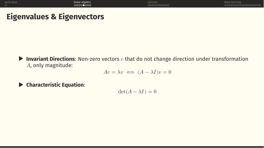
An eigenvector is a non-zero vector $v$ that the matrix $A$ does not rotate, it only stretches or shrinks. The stretch factor $λ$ is the eigenvalue.

What it means

Most vectors, when you multiply them by a matrix, get pushed off in some new direction. Eigenvectors are the exception: they lie along axes the transformation "believes in", and along those axes it behaves like plain multiplication. Finding them reduces to solving a polynomial, the characteristic equation.

A v = λ v \Leftrightarrow (A - λ I) v = 0

→ where this goes

Eigenvectors of symmetric matrices are orthogonal, and their eigenvalues are the squared singular values of the SVD. So every time later slides say "singular values", they mean "square roots of the eigenvalues of $A^{T} A$ ." Keep this in your back pocket for page 40.

Page 08 / 82

$Low-rank matrices via outer products. uv^T has rank 1. Sum of r rank-1 matrices = BA with B (d×r) and A (r×k), r ≪ min(d,k). Parameter cost r(d+k) instead of d·k.$

page 08 · outer products & rank

On the slide

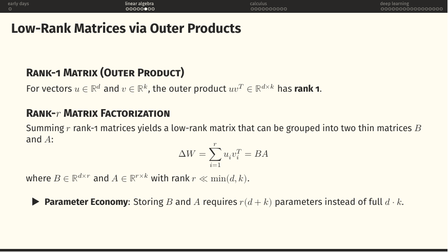
Take two vectors $u$ and $v$ . Their outer product $u v^{T}$ is a matrix, but a very poor matrix, in the sense that every column is a scalar multiple of $u$ . It has rank 1. Sum $r$ of these and you get a matrix of rank at most $r$ .

What it means

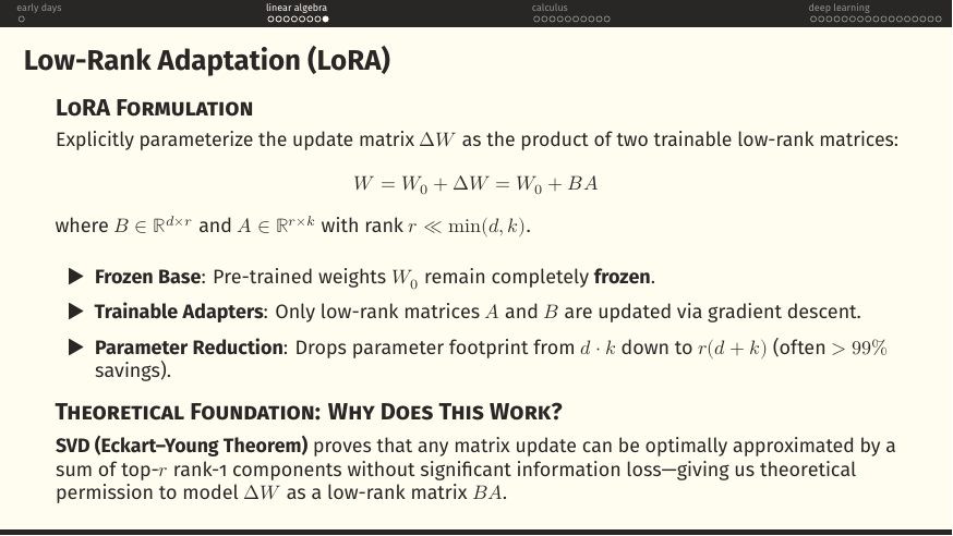
A dense $d \times k$ matrix stores $d k$ numbers. If we know in advance that the matrix has rank $r$ , we can factor it as $B A$ with $B$ tall-and-thin and $A$ short-and-wide, and pay only $r (d + k)$ numbers. When $r ≪ \min (d, k)$ , that is a huge saving. This is the entire reason low-rank adaptation exists.

Page 09 / 82

$The LLM fine-tuning bottleneck. Full fine-tuning updates W = W0 + ΔW; ΔW has d·k parameters per matrix; intrinsic rank hypothesis says the essential update lives in a low-dim subspace.$

page 09 · the bottleneck

Page 10 / 82

$LoRA. Parameterise ΔW = BA with B (d×r), A (r×k). Freeze W0, train only A and B. Eckart–Young / SVD justifies why a low-rank ΔW is enough.$

page 10 · LoRA

On these slides

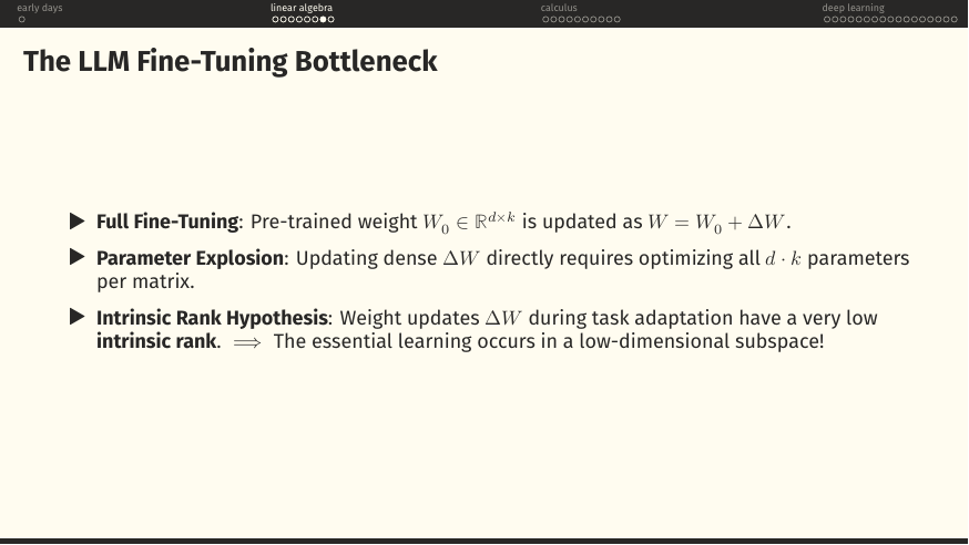
The problem: a modern language model's weight matrix $W_{0}$ is huge, think $4096 \times 4096$ , and updating it directly means training sixteen million parameters per matrix, per task. The intrinsic rank hypothesis observes empirically that the update $Δ W$ a task needs is nowhere near that rich. It lives in a much smaller subspace.

The idea behind LoRA

Freeze $W_{0}$ . Parameterise the update as $Δ W = B A$ with rank $r$ (typically 4, 8, or 16). Train only $A$ and $B$ . Parameter count drops from $d \cdot k$ to $r (d + k)$ , which is more than 99% savings for realistic sizes. The theoretical cover is the Eckart-Young theorem: for any matrix, the best rank- $r$ approximation is given by keeping the top $r$ singular components of its SVD. So if the true update was low-rank all along, we lose essentially nothing.

✦ the aha

Every fact about linear algebra you have accumulated across pages 4-8 is deployed on this one page. Vectors and their outer products (page 8) give you the rank-1 pieces; SVD (page 6, one line about "rotate-scale-rotate") tells you those pieces are optimal; the intrinsic-rank observation says nature is being generous. LoRA is not clever, it is just reading linear algebra correctly.

§3Calculus: from derivatives to Muon

Thirty-three pages, and every one of them earns its space. The move is escalation: scalar functions of one variable (page 12), then many variables (17), then vector-valued functions (25), then second derivatives that live in a matrix (29). Once we have the machinery we spend the rest of the section using it, first to walk downhill (gradient descent), then to walk downhill more cleverly (Newton-Raphson), then to hint at a very modern optimizer that uses the SVD trick from §2. If you only take one section of this tutorial seriously, take this one.

Page 11 / 82

$Section divider: Calculus.$

page 11 · section divider

The second big sweep of the tutorial opens.

Page 12 / 82

$Why would you differentiate matrices? First principles: limit as Δx→0 of (f(x+Δx)−f(x))/Δx.$

page 12 · first principles

Page 13 / 82

$Fair enough: derivative of a matrix of scalar functions is the matrix of derivatives, entrywise.$

page 13 · differentiate entrywise

On these slides

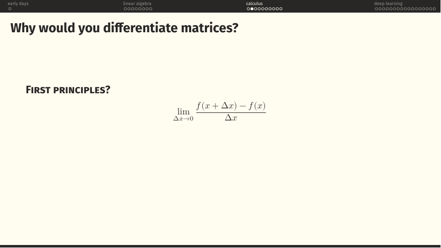
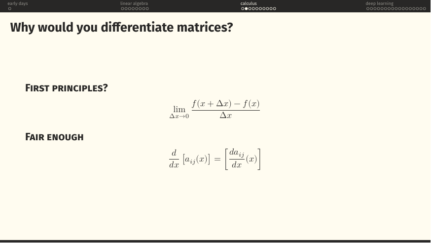
A gentle onboarding to the section's central question, how do we differentiate a matrix? Page 12 reminds you what a derivative is at all: the limit of a rise-over-run as the run goes to zero. Page 13 gives the honest, boring answer to the matrix question: if a matrix's entries are all scalar functions $a_{i j} (x)$ , then its derivative is just the matrix whose entries are the individual derivatives $\frac{d a_{i j}}{d x}$ .

Why start here

The rest of the tutorial is going to bend the definition of "derivative" in progressively weirder directions, with respect to a vector, then with respect to a matrix, then with respect to a whole neural network's parameter tensor $Θ$ . If the very first move (differentiating a matrix of scalar functions elementwise) doesn't sit comfortably, the later moves won't either.

"Why are there so many variables?": partial derivatives

Page 14 / 82

$How would you differentiate a multivariable function?$

page 14 · the question

Page 15 / 82

$Example: f(x,y) = x² + y² + 2xy.$

page 15 · the example

Page 16 / 82

$Naive intuition says df/dx = 2x + 2y; 12th-grade calculus, treating y as a function of x, says df/dx = (2x+2y)(1 + dy/dx).$

page 16 · the paradox

Page 17 / 82

$The resolution: partial derivatives.$

page 17 · the resolution

Page 18 / 82

$∂f/∂x is the derivative when every other variable is held constant.$

page 18 · the definition

What this build shows

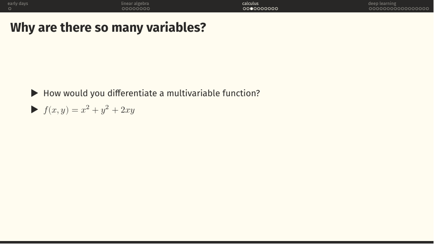
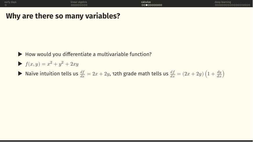
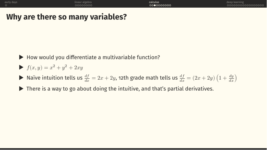
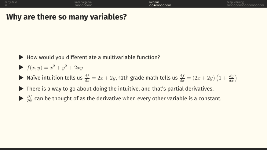
The five slides pose the same puzzle and then pull the rabbit out. If $f (x, y) = x^{2} + y^{2} + 2 x y$ , is $\frac{d f}{d x}$ equal to $2 x + 2 y$ , or does it need a $d y / d x$ correction? The two 12th-grade instincts disagree.

What it means

They disagree because $d f / d x$ is an underspecified question when there are two independent variables. The fix is the partial derivative $\partial f / \partial x$ : differentiate with respect to $x$ while pretending every other variable is a constant. For our $f$ , that gives $\partial f / \partial x = 2 x + 2 y$ . Cleanly.

◉ mental model

Picture $f (x, y)$ as a hilly landscape over the $x - y$ plane. $\partial f / \partial x$ is the slope you would feel if you took a step in the pure $x$ direction. $\partial f / \partial y$ is the slope in the pure $y$ direction. Each partial ignores the other axis on purpose.

"Dear Lord, it's Physics!": the gradient

Page 19 / 82

$It makes sense to consider components of a derivative along the coordinate axes.$

page 19 · components

Page 20 / 82

$Each component must be ∂f/∂x_i.$

page 20 · the components are partials

Page 21 / 82

$Voilà: ∇f = [∂f/∂x_i]^T, or, for physicists, ∇f = Σ ∂f/∂x_i · x̂_i.$

page 21 · the gradient

What this build shows

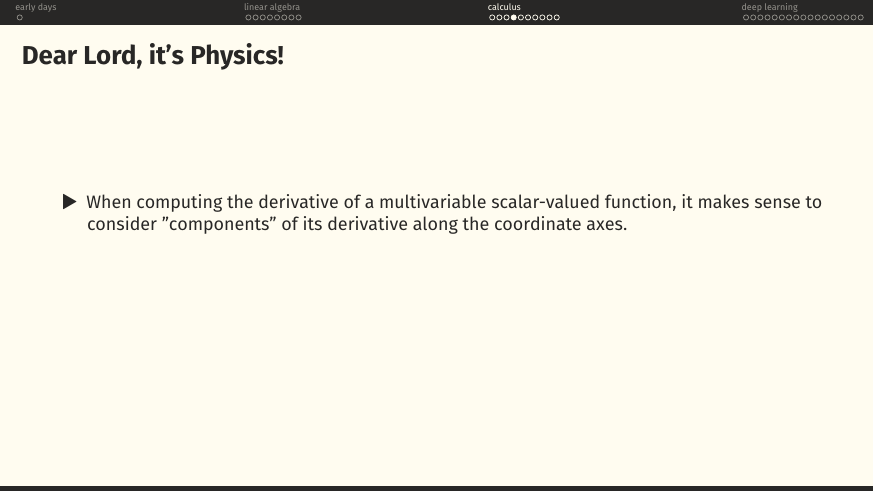
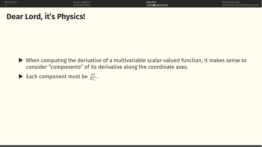
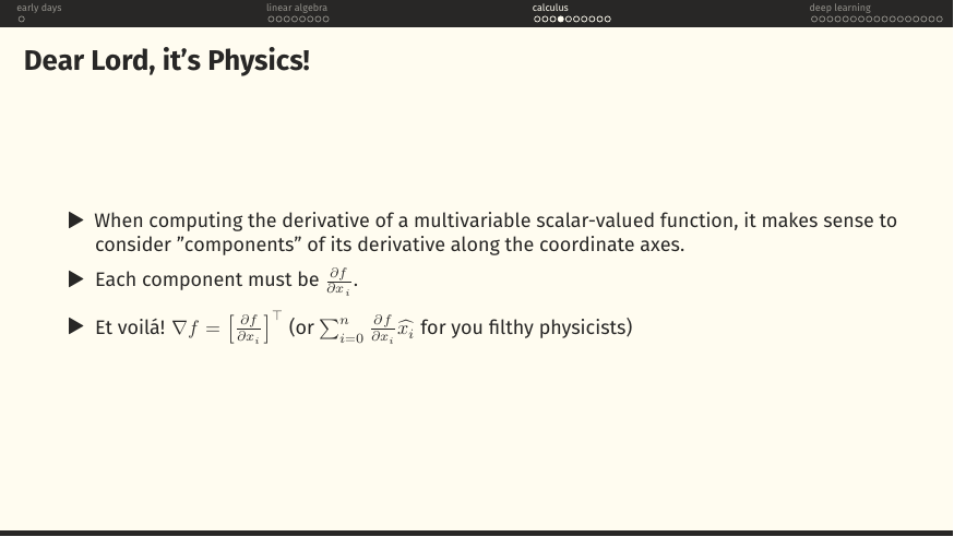
Package all the partial derivatives of a scalar-valued $f : ℝ^{n} \to ℝ$ into a single object. The result is a vector.

What it means

That vector is the gradient $\nabla f$ . It has one entry per input coordinate, and each entry is the partial derivative along that coordinate. Geometrically it points uphill in the steepest direction, and its length is the steepness of that steepest ascent.

\nabla f = {[\frac{\partial f}{\partial x_{1}} \frac{\partial f}{\partial x_{2}} \dots \frac{\partial f}{\partial x_{n}}]}^{T}

✦ the aha

The title's joke is real. Physicists write the same object as $\nabla f = \sum_{i} \frac{\partial f}{\partial x_{i}} {\hat{x}}_{i}$ , using unit-vector notation. Mathematicians stack the components in a column and call it a day. Same beast either way.

"Corn on the Jacob": the Jacobian

Page 22 / 82

$For f: ℝ^n → ℝ^m, how would you deal with df/dx?$

page 22 · the question

Page 23 / 82

$You need derivatives of every output y_i wrt every input x_j.$

page 23 · every-with-every

Page 24 / 82

$That is mn possible values.$

page 24 · mn possibilities

Page 25 / 82

$Assemble them into the Jacobian matrix J = [∂y_i / ∂x_j].$

page 25 · the Jacobian

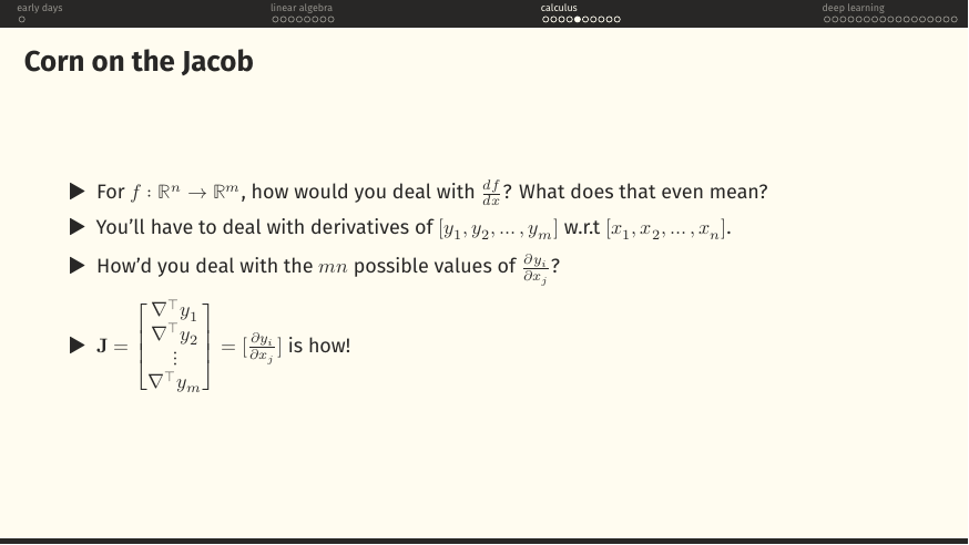
What this build shows

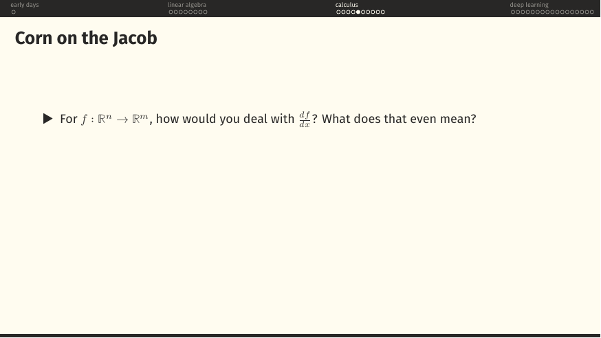
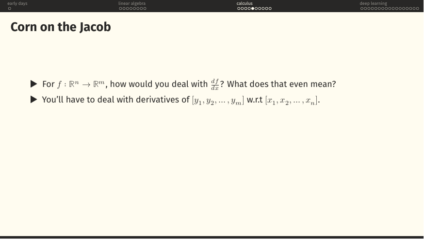
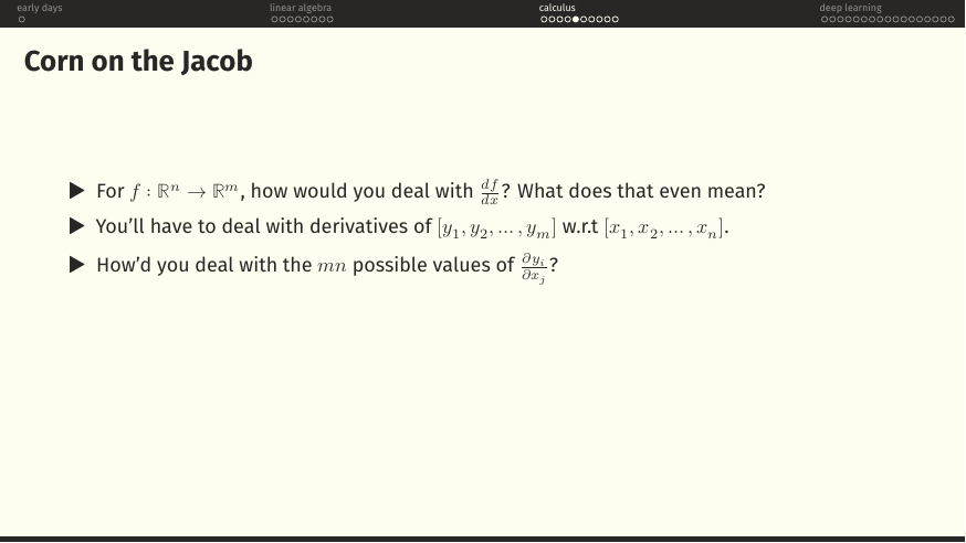
The gradient handled a scalar output. What if the output is itself a vector? Then a single "derivative" is not enough, you need one number for every combination of output and input coordinate. That is $m \times n$ numbers.

What it means

Stack them in a matrix. The Jacobian $J$ has one row per output coordinate, that row is the gradient (transposed) of that output. It has one column per input coordinate. Entry $(i, j)$ is $\partial y_{i} / \partial x_{j}$ . If you feed the Jacobian a small displacement $δ x$ , it hands you back the best linear estimate of the resulting $δ y$ . The Jacobian is the derivative, generalised.

◉ dimensions cheat sheet

Given $f : ℝ^{n} \to ℝ^{m}$ : the Jacobian is $m \times n$ . If $m = 1$ (scalar output), $J$ collapses to $(\nabla f)^{T}$ . If $n = 1$ (scalar input), it collapses to the ordinary derivative vector. Every subsequent Jacobian in this course will fall into one of these two shapes.

"We've had one breakfast, yes…": the Hessian

Page 26 / 82

$What about second derivatives? Useful for finding extrema, and for one more thing later.$

page 26 · second breakfast

Page 27 / 82

$For scalar f, we saw ∇f: ℝ^n → ℝ^n.$

page 27 · gradient is vector-valued

Page 28 / 82

$So take its Jacobian: J∇f = [∂²f/(∂x_j ∂x_i)].$

page 28 · Jacobian of the gradient

Page 29 / 82

$By convention, use the transpose: H = (J∇f)^T. This is the Hessian.$

page 29 · the Hessian

What this build shows

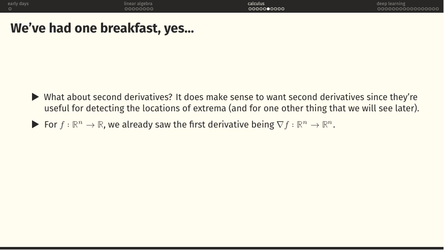
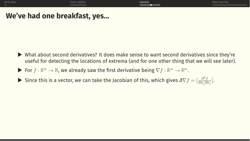
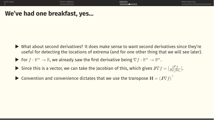
Second derivatives. For a scalar-valued $f$ , the first derivative is a vector (the gradient); the derivative of that vector is a matrix, the Hessian $H$ . Entry $(i, j)$ is $\partial^{2} f / \partial x_{i} \partial x_{j}$ , the sensitivity of the $i$ -th partial to a wiggle in the $j$ -th input.

What it means

Second derivatives tell you about curvature. In 1D, positive $f^{''}$ means the graph is cupping upward, you are near a minimum, not a maximum. In many variables the same information lives in the eigenvalues of $H$ : all-positive means a local min, all-negative means a local max, mixed signs means a saddle. Second derivatives are also the "one other thing" hinted at, they will show up in Newton-Raphson two pages later.

✦ the aha

The convention $H = (J \nabla f)^{T}$ is not arbitrary. Because mixed partials commute for nice functions (Clairaut / Schwarz), $H$ is symmetric, a fact that will save your life every time you want to invert one.

Page 30 / 82

$Consider being on a hill wanting to reach the lowest point. A local minimum will do. You can only see where you are and the local shape of the ground. How do you get down?$

page 30 · the hill

On the slide

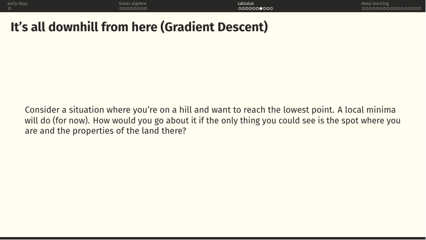
The core parable of optimisation. You are somewhere on a landscape, blindfolded except for a small patch of ground around your feet. Your job is to get to the lowest point you can. What do you do?

What it means

Feel the slope, take a step downhill, repeat. This is gradient descent. Formally, if the landscape's height is $f (x)$ , the direction of fastest ascent is $\nabla f$ , so the direction of fastest descent is $- \nabla f$ . Step size is a hyperparameter you get to pick.

x_{k + 1} = x_{k} - η \cdot \nabla f (x_{k})

⚠ common trap

The phrase "a local minimum will do (for now)" is doing enormous work. Gradient descent finds a minimum, not the minimum. The whole reason deep-learning practitioners obsess over initialisation, learning-rate schedules, and momentum is that the local minimum you land in depends on where you started and how you walked.

Newton-Raphson: walking downhill using curvature

Page 31 / 82

$Given f: ℝ→ℝ, iteratively compute the minima.$

page 31 · the problem

Page 32 / 82

$Construct a sequence {x_i} converging to argmin f.$

page 32 · a sequence

Page 33 / 82

$Second-order Taylor: f(x_k + t) ≈ f(x_k) + f'(x_k)t + ½ f''(x_k) t².$

page 33 · Taylor around x_k

Page 34 / 82

$Minimize this local approximation — set its derivative to zero.$

page 34 · set derivative to zero

Page 35 / 82

$0 = f'(x_k) + f''(x_k) t.$

page 35 · solve for t

Page 36 / 82

$x_{k+1} = x_k − f'(x_k)/f''(x_k). Newton-Raphson.$

page 36 · the update

Page 37 / 82

$For f: ℝ^n → ℝ, the update is x_{k+1} = x_k − ∇f · H^{−1}.$

page 37 · multivariate Newton

What this whole build shows

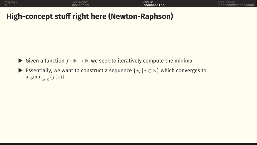
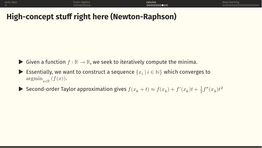
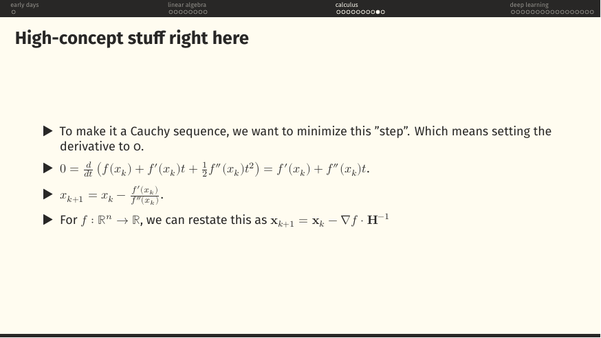
A more principled hill-descent than gradient descent. Instead of just following the slope, we build a quadratic model of the landscape at our current point, using the value, the slope, and the curvature, and jump directly to that model's minimum. Iterate.

What it means

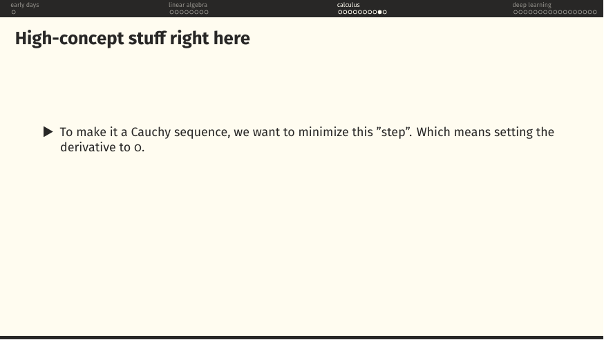
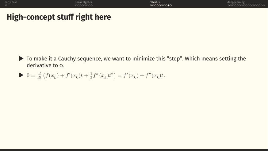
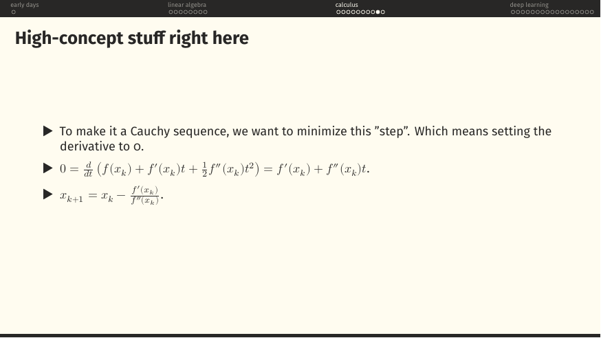
Second-order Taylor says $f (x_{k} + t) \approx f (x_{k}) + f^{'} (x_{k}) t + \frac{1}{2} f^{″} (x_{k}) t^{2}$ . Minimise the right-hand side in $t$ : differentiate, set to zero, solve. You get the Newton-Raphson step $x_{k + 1} = x_{k} - f^{'} (x_{k}) / f^{″} (x_{k})$ .

In many variables the same story becomes $x_{k + 1} = x_{k} - H^{- 1} \cdot \nabla f$ , you pre-multiply the gradient by the inverse of the Hessian.

⚠ why nobody uses this at scale

The multivariate update needs $H^{- 1}$ . For a modern network with $N = 10 10^{}$ parameters, the Hessian is $N \times N$ . Storing it is a nonstarter; inverting it is science fiction. This is exactly why the next few pages are about first-order tricks that approximate curvature without ever writing $H$ down.

"If at first you don't succeed…": a preview of Muon

Page 38 / 82

$Modern methods use linear transformations that parallelise well (thanks, Vaswani et al!).$

page 38 · parallelisable

Page 39 / 82

$For reasons, we can try to push a matrix's nonzero singular values towards 1.$

page 39 · nudge singular values → 1

Page 40 / 82

$Odd polynomials commute with the SVD: p(UΣV^T) = U p(Σ) V^T.$

page 40 · SVD-commuting

Page 41 / 82

$There exist odd polynomials p: ℝ→ℝ with lim_{n→∞} p^n(x) = sgn(x), at least near 0.$

page 41 · p^n(x) → sgn(x)

Page 42 / 82

$So picking the right coefficients gives a good enough approximation.$

page 42 · pick coefficients

Page 43 / 82

$This is a surprise tool which will help us later.$

page 43 · a surprise tool

What this build shows

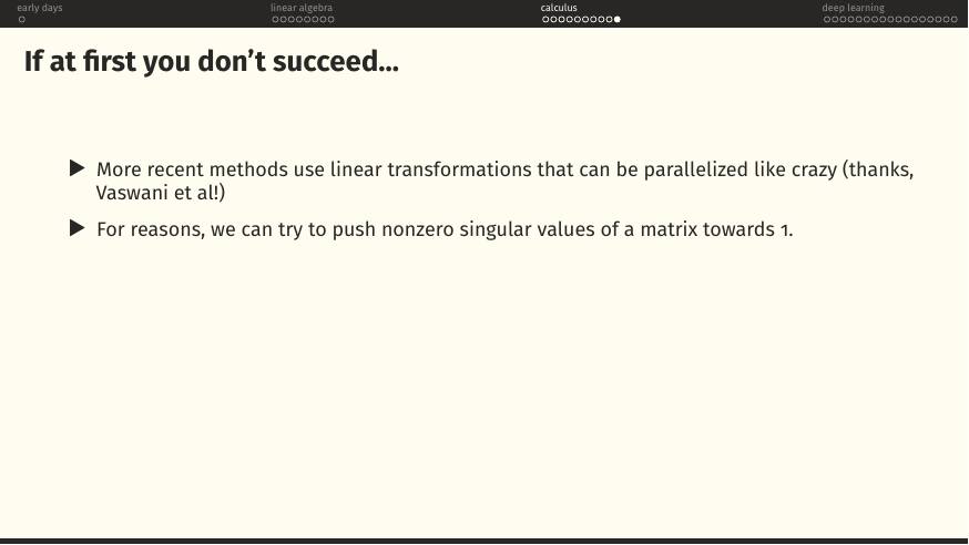
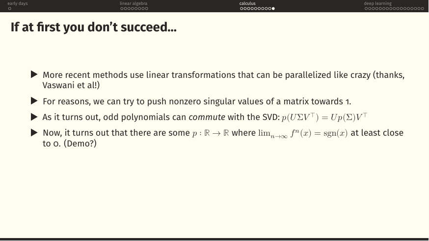
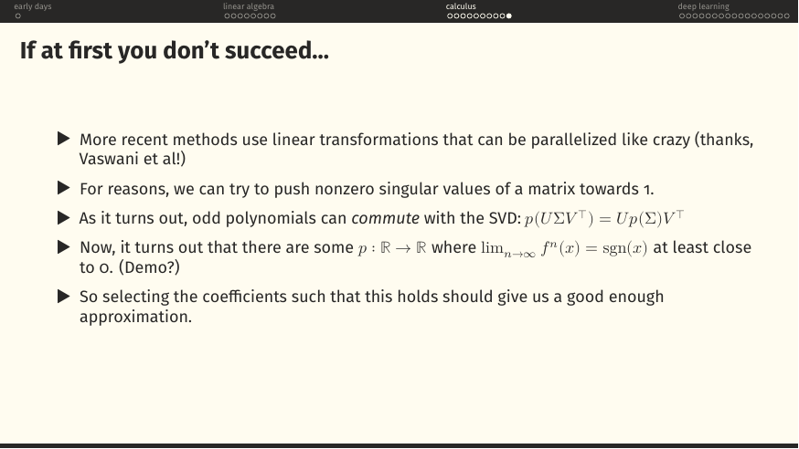
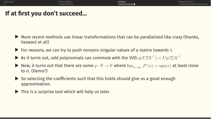
A six-slide teaser for something that will land, in full, at the end of §4. The story: modern optimisers need updates that are matrices, and those updates would be more well-behaved if the matrix had all singular values equal to 1, that is, if it were pushed toward an orthogonal matrix (recall page 6). How do you do that on a GPU without ever calling the SVD?

The trick

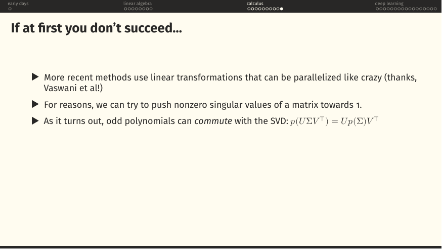
Odd polynomials, think $p (x) = 3 x - 3 x^{3} + x^{5}$ , have a magical property: $p (U Σ V^{T}) = U p (Σ) V^{T}$ . Applying the polynomial to the whole matrix is the same as applying it to each singular value in isolation. So if we can find a polynomial $p$ such that iterating $p$ on any real number in $(0, ∞)$ converges to 1, then iterating $p$ on any matrix will drive all its singular values to 1, without ever computing the SVD explicitly. Only matrix multiplies, which GPUs adore.

→ payoff at page 75

This is called Newton-Schulz iteration, and it is the beating heart of the Muon optimizer, which shows up at the very end of the deep-learning section. When you get there, remember these six pages, they are the whole reason Muon works at all.

§4Deep learning: assembling the machine

Thirty-nine pages, and the payoff for everything before. Deep learning is now defined in one sentence: pick a parametrised function and tune the parameters until it does what you want. The section justifies why such a function even exists (Universal Approximation), gives it teeth (classification, softmax), and then explains how to actually find the parameters using every tool from §3 (loss functions, chain rule, backprop, SGD, Adam, and finally Muon). By the last page you have built a language model from first principles.

Page 44 / 82

$Section divider: Deep Learning.$

page 44 · section divider

The final and longest sweep.

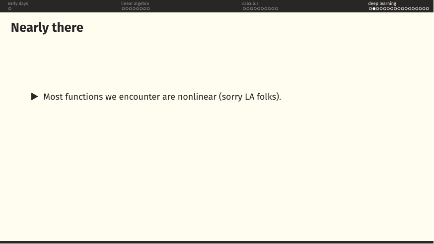
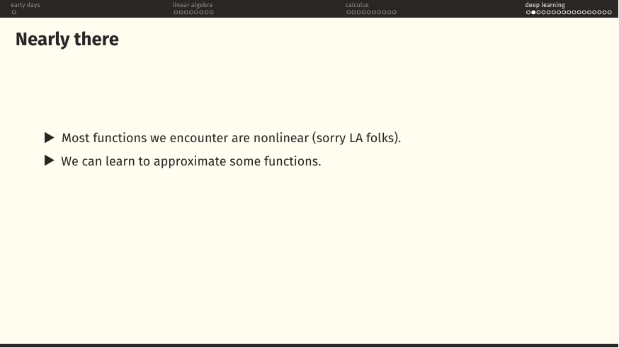
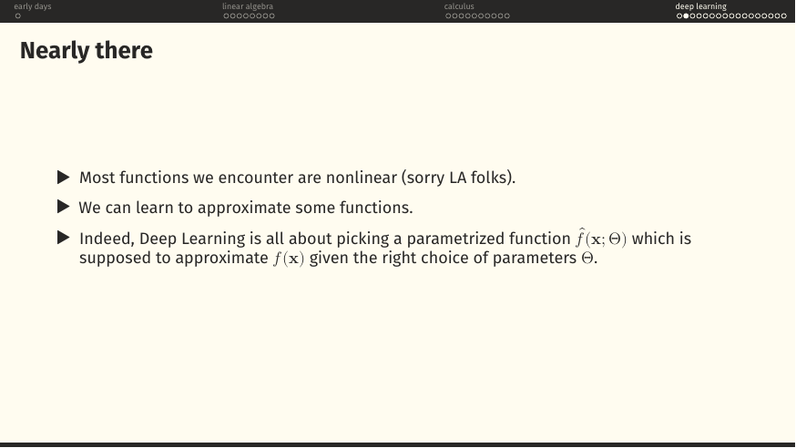
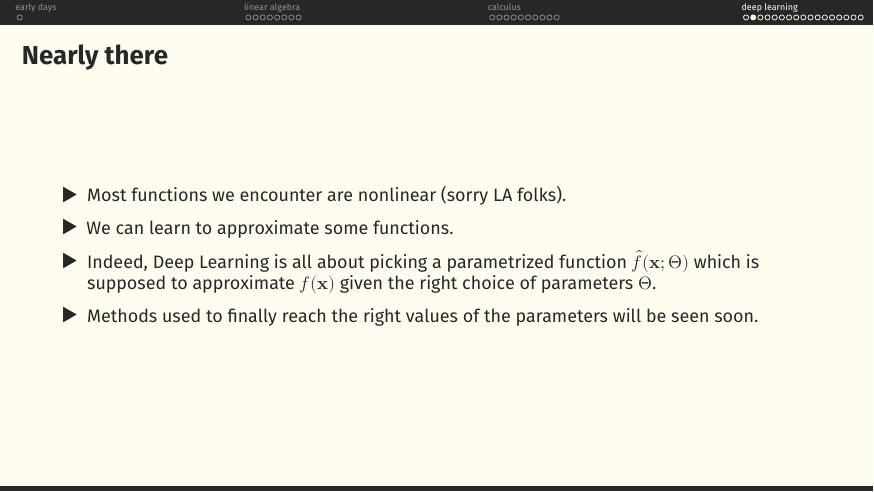
"Nearly there": deep learning in one sentence

Page 45 / 82

$Most functions we encounter are nonlinear (sorry LA folks).$

page 45 · reality is nonlinear

Page 46 / 82

$We can learn to approximate some functions.$

page 46 · approximate them

Page 47 / 82

$Deep learning: pick a parameterised f̂(x; Θ) approximating the true f(x).$

page 47 · the definition

Page 48 / 82

$Methods for finding the right Θ will be seen soon.$

page 48 · finding Θ, later

What this build shows

The definition of deep learning, unpacked slowly. The world is full of functions we care about, from images to labels, from English to French, from prompt to next token, and most of them are not linear. So we pick a family of parametrised functions $\hat{f} (x; Θ)$ , flexible enough to plausibly contain a good approximation of the target $f (x)$ , and we search over $Θ$ for the setting that best fits the data.

◉ what Θ actually is

$Θ$ is every tunable number in the network, all the weight matrices $A_{i}$ , all the bias vectors $b_{i}$ , all the layer-norm scale factors, all the embedding entries. For a 7B model that is seven billion numbers. Section §3 is going to earn its rent here.

Classification: slicing space with hyperplanes

Page 49 / 82

$Treat n-way classification as f: ℝ^m → ℝ^n where outputs form a probability distribution over classes.$

page 49 · classification as a function

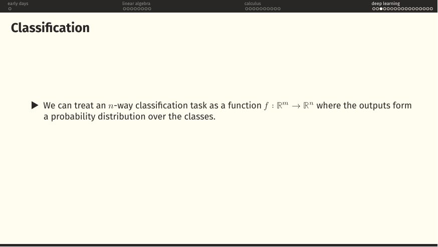
The first concrete instance of the parametrised-function view: classification. Input an $m$ -dimensional feature vector, output an $n$ -dimensional vector of class probabilities. Whichever entry is largest, that is the model's prediction.

Page 50 / 82

$Equivalently: draw (n−1) (m−1)-hyperplanes that split m-space into n pieces.$

page 50 · hyperplanes as decision surfaces

Page 51 / 82

$Grid of red and green dots with a horizontal line separating them. Caption: pretty straightforward to slice.$

page 51 · easy case

Page 52 / 82

$Grid with a diagonal split still separating red and green. Caption: still straightforward to slice.$

page 52 · still easy

Page 53 / 82

$XOR pattern of red and green points: no single line separates them. Caption: oh no.$

page 53 · XOR: oh no

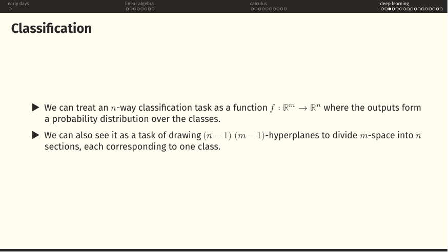
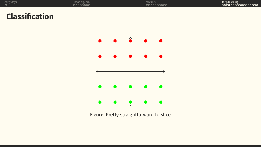
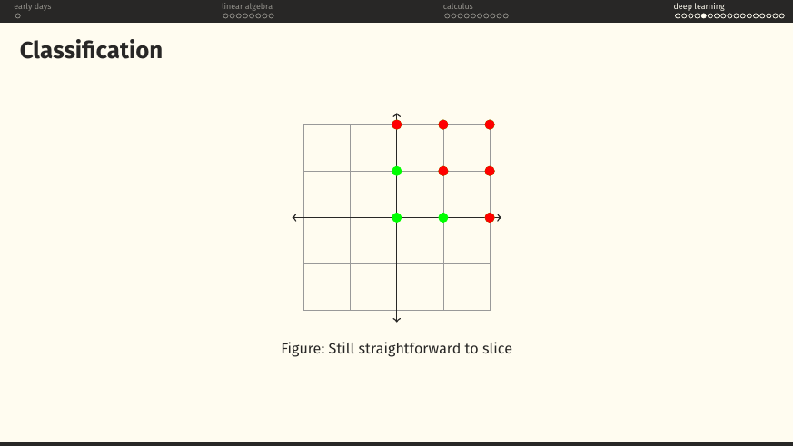
What this build shows

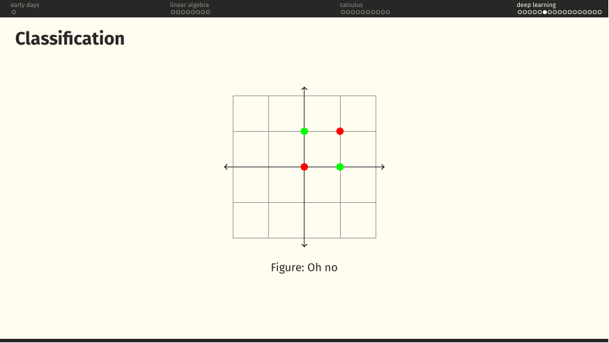
The geometry of classification. Splitting an $m$ -dimensional input space into $n$ class regions is the same as drawing $n - 1$ hyperplanes (lines in 2D, planes in 3D, etc). For "nice" data, the first two grids, one straight line does it. Then comes XOR: red at NE and SW, green at NW and SE. No single straight line separates them.

✦ the aha

This "oh no" moment is exactly why the field spent a decade after 1969 in the neural-net winter. Minsky and Papert showed that a single-layer perceptron cannot solve XOR. The fix, hinted at on the very next pages, is composition with a nonlinearity: bend the input space before you try to cut it, and the problem becomes linearly separable in the bent space.

"Ain't linear no mo": why we need nonlinearities

Page 54 / 82

$Consider A_1(A_2(⋯) + b_2) + b_1 — a composition of affine maps.$

page 54 · composing affine maps

Page 55 / 82

$But that just equals A' x + b' for some A', b'. Composing affine gives you affine.$

page 55 · still affine

Page 56 / 82

$Introduce a nonlinearity: f_i(x) = f(A_i x + b_i), then compose f_1(f_2(f_3(⋯))).$

page 56 · add σ, get real

What this build shows

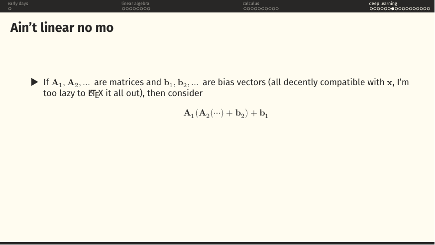
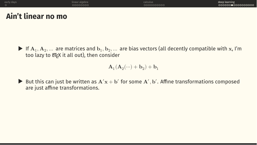
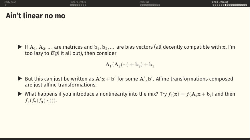
Why simply stacking linear layers is useless, and what fixes it. Composing two affine maps $x \mapsto A_{1} (A_{2} x + b_{2}) + b_{1}$ collapses algebraically to a single affine map $A^{'} x + b^{'}$ . A hundred layers deep, still one affine map. XOR still unsolvable.

The fix: sandwich a pointwise nonlinearity $σ$ between the layers. Now the composition $f_{1} \circ f_{2} \circ f_{3} \circ \dots$ is a genuinely new function that cannot be flattened. This is why every deep network, from a 1990s MLP to a 2026 transformer, has ReLU, GELU, SiLU, or some other pointwise squish between its linear layers.

Page 57 / 82

$Universal Approximation Theorem: for any continuous f: K → ℝ^m on compact K and any ε>0, there exist A_1, A_2, b such that sup_{x∈K} ‖f(x) − A_2 σ(A_1 x + b)‖ < ε.$

page 57 · Universal Approximation

On the slide

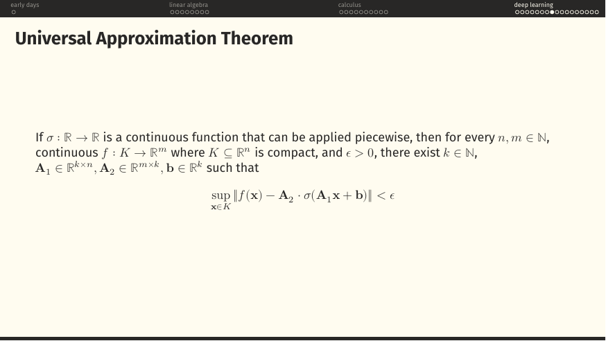
The Universal Approximation Theorem, stated formally. In plain English: given any continuous function on a bounded region, and any tolerance you like, there exists a two-layer network, one linear layer, one nonlinearity, one more linear layer, that agrees with your target function everywhere in the region to within that tolerance.

◉ what the theorem does and does not promise

Does promise: such a network exists. Does not promise: you can find its weights with gradient descent, or that the required width $k$ is small, or that the network generalises to unseen data. UAT is an existence result, not a training guarantee.

Page 58 / 82

$Universal Approximation Theorem (abridged): any continuous function can be approximated by a 2-layer perceptron with arbitrary precision.$

page 58 · UAT, abridged

Page 59 / 82

$Universal Approximation Theorem (proof): a cartoon of a unicorn.$

page 59 · uhhhh here's a unicorn

What these two show

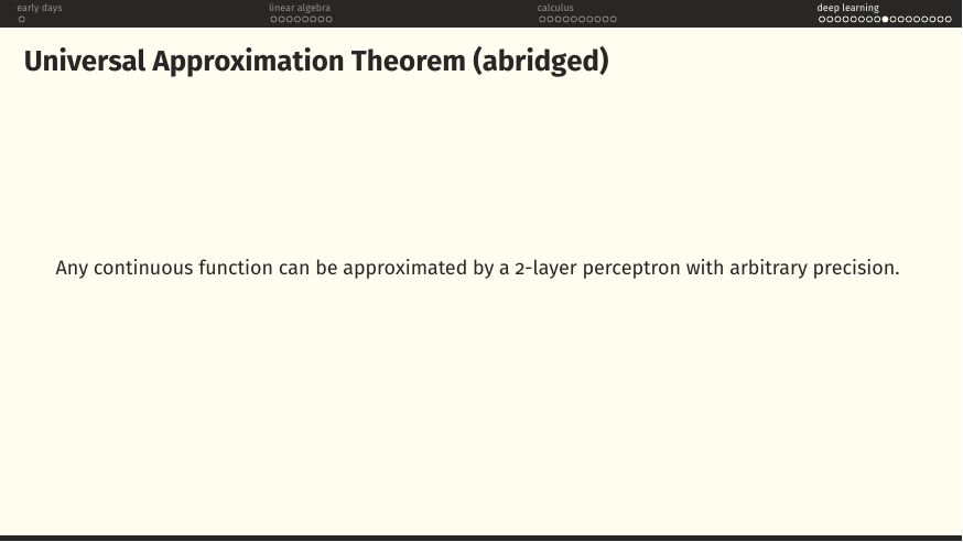
The abridged theorem strips off the epsilons and just says: any continuous function can be approximated by a two-layer network as closely as you like. The next slide, mock-titled "proof", presents a unicorn.

✦ the aha (the joke)

The joke is that the actual proof (Cybenko 1989, Hornik 1991) is a densely functional-analytic argument involving the Hahn-Banach theorem and the Riesz representation theorem. Nobody wants to reproduce that on a tutorial slide. The unicorn stands in for a proof exactly the way "left as an exercise for the reader" does in textbooks, with the added candour of admitting that it exists more in the imagination than in your notebook right now.

"Begging the question 101": the loss

Page 60 / 82

$So far we've assumed the correct weights are chosen by some oracle. How do we get them IRL?$

page 60 · but who picks Θ?

Universal approximation guarantees the right $Θ$ exists. It says nothing about how to find it. That is the question the rest of the section answers.

Page 61 / 82

$We know what we want and what the model gives — find a metric to compare them.$

page 61 · we need a metric

Page 62 / 82

$Cross-entropy loss: L(f̂(x;Θ), f(x)) = − Σ y_i log(ŷ_i).$

page 62 · cross-entropy loss

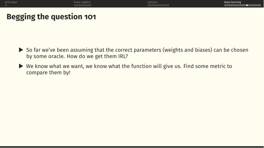
What this build shows

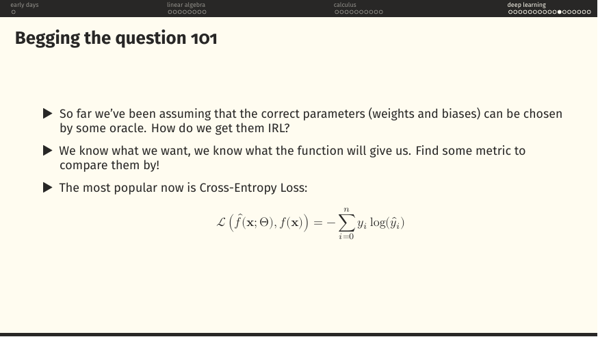
Define a loss function $L$ that measures how wrong the model is. The cross-entropy loss, the standard for classification and language modelling:

L (\hat{f} (x; Θ), f (x)) = - \sum_{i = 0}^{n} y_{i} \log ({\hat{y}}_{i})

where $y_{i}$ is 1 for the correct class and 0 otherwise, and ${\hat{y}}_{i}$ is the model's predicted probability for class $i$ . When the model is confident and right, $\log (\hat{y})$ is close to 0 and the loss is small. When it is confident and wrong, $\log (\hat{y})$ heads to $- \infty$ and the loss explodes. That asymmetry, being punished more for being confidently wrong than for being timidly wrong, is the whole point.

→ where this goes

Training the model = choosing $Θ$ to minimise $L (Θ)$ . That is a many-variable minimisation problem. §3 has already taught you how to attack it, gradient descent needs $\nabla_{Θ} L$ . The next five pages compute that gradient.

Chain rule: the same slides twice, once for chain rule and once for backprop

Page 63 / 82

$Chain rule clutch, as always. Θ is not a matrix — how do we differentiate wrt each parameter?$

page 63 · the setup

Page 64 / 82

$For a 1D perceptron f̂ = f(ax+b), ∂L/∂a = (∂L/∂f̂)(∂f̂/∂(ax+b))(∂(ax+b)/∂a).$

page 64 · one perceptron, one weight

Page 65 / 82

$Similarly obtain ∂L/∂x and ∂L/∂b.$

page 65 · same idea for x, b

Page 66 / 82

$More than one layer: reuse ∂L/∂x with x = output of the previous layer. Chain rule applies again.$

page 66 · deeper networks

Page 67 / 82

$This scales over perceptron dimensions (verify!).$

page 67 · and over widths

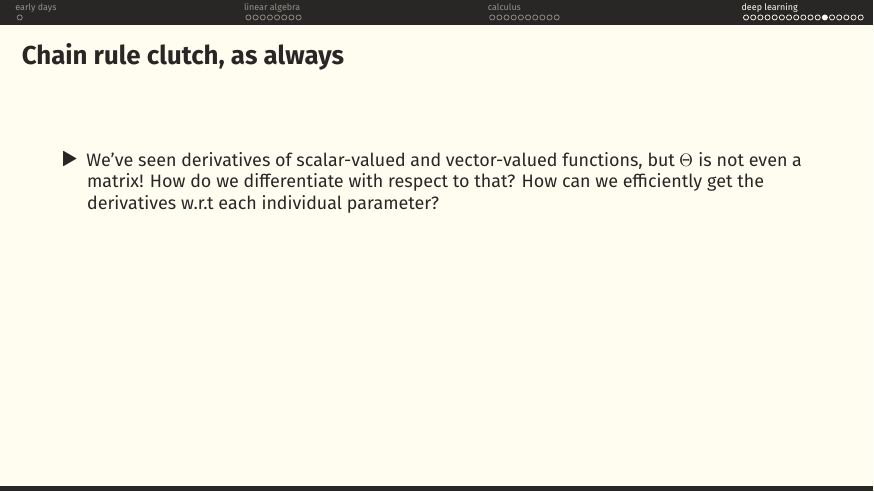
What this build shows

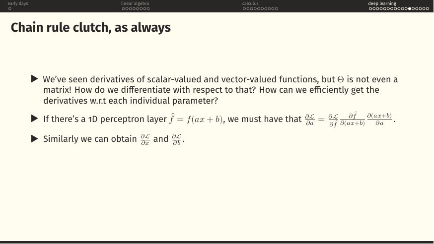
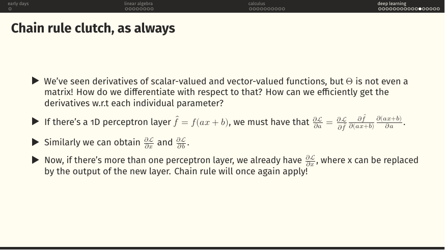
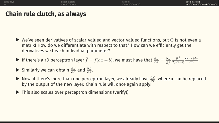
How the chain rule, learned in high school, is enough to compute the gradient of the loss with respect to every parameter in a network, no matter how deep, no matter how wide.

What it means

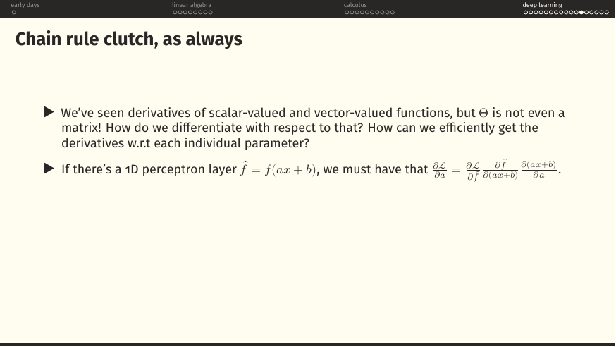
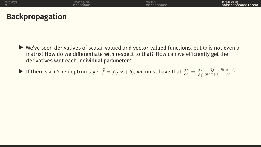
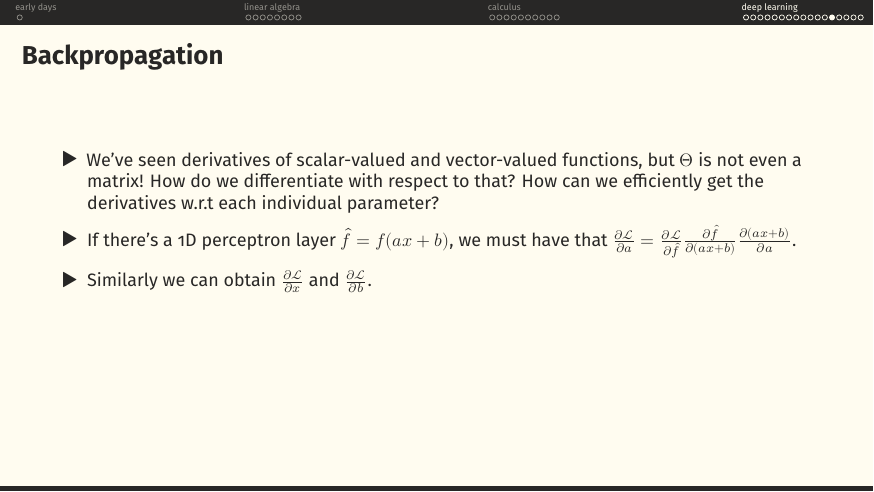
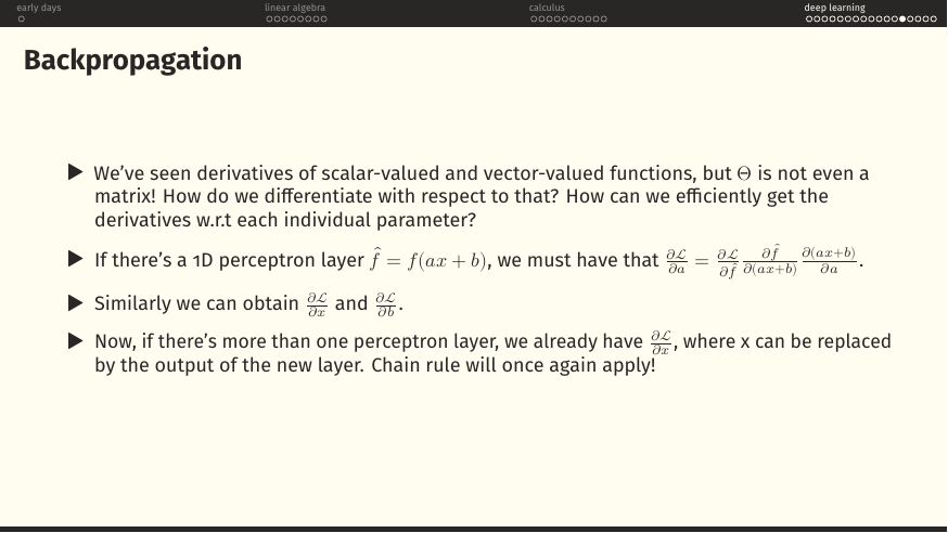
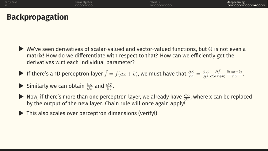
For a single-perceptron model $\hat{f} = f (a x + b)$ , the loss depends on $a$ through a chain of three steps: $a$ enters the pre-activation $a x + b$ , which passes through the nonlinearity $f$ to produce $\hat{f}$ , which enters $L$ . Multiply the three local derivatives together. Same argument works for $x$ and $b$ . And for deeper networks: the $\partial L / \partial x$ you just computed is exactly the "loss gradient" the previous layer needs, plug it in as the starting point of a fresh chain-rule expansion.

◉ why "chain rule" and "backprop" are the same slides

Because they are the same idea, phrased twice. Chain rule tells you the mathematical fact; backprop tells you how to compute it efficiently, right-to-left, layer by layer, reusing the downstream gradient as you go. The next five slides restate the same content under the label "Backpropagation" to hammer this home.

Backpropagation: the same idea, with a computer in mind

Page 68 / 82

$Backpropagation setup.$

page 68 · restatement

Page 69 / 82

$Backprop for a 1D perceptron.$

page 69 · one perceptron

Page 70 / 82

$Backprop wrt x and b.$

page 70 · same for x, b

Page 71 / 82

$Backprop through more layers.$

page 71 · deeper

Page 72 / 82

$Backprop scales over perceptron dimensions (verify!).$

page 72 · and wider

On the slide

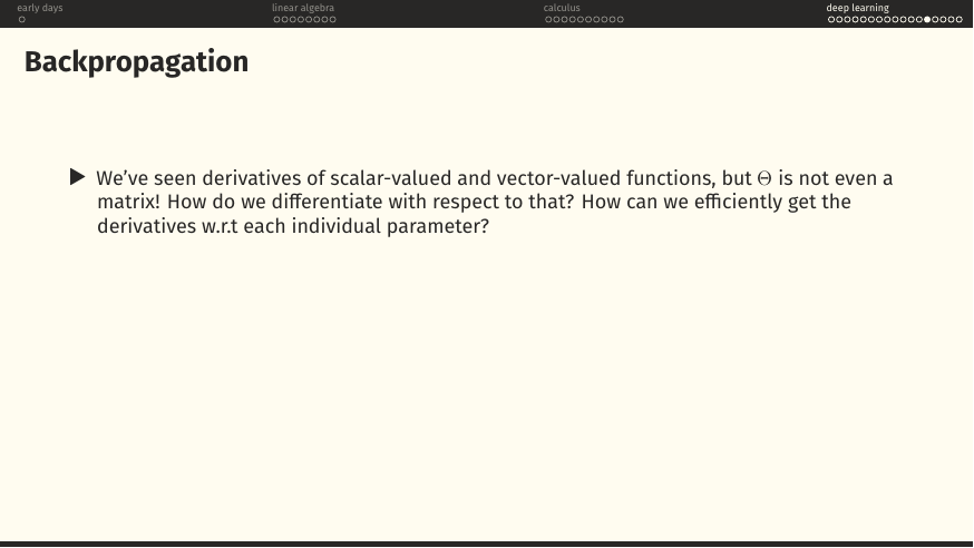
The exact same five slides, one word swapped: "chain rule" → "backpropagation". The deliberate repetition is the pedagogy.

What it means

Backpropagation is what you get when you commit to computing the chain-rule gradients in a specific order: start at the loss (the top of the network), compute $\partial L / \partial (output)$ , and walk backwards through the layers, at each step turning "gradient with respect to this layer's output" into "gradient with respect to this layer's parameters" and "gradient with respect to this layer's input". The second output becomes the first input for the layer below.

✦ the aha

Nothing is happening here that wasn't already in the chain rule. What backprop adds is dynamic programming: instead of re-deriving the gradient from scratch for every parameter, you compute the shared intermediate quantities once and reuse them. On a modern network with a billion parameters, this is the difference between minutes and centuries.

Optimisers: from SGD to Muon

Page 73 / 82

$Stochastic gradient descent minimises L wrt Θ: θ_{k+1} = θ_k − η · ∇_θ L.$

page 73 · SGD

Page 74 / 82

$SGD with Momentum, Adam and AdamW are better approaches to the same principle.$

page 74 · momentum, Adam, AdamW

What this build shows

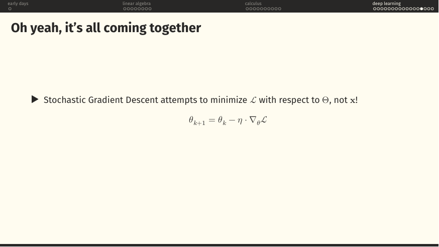
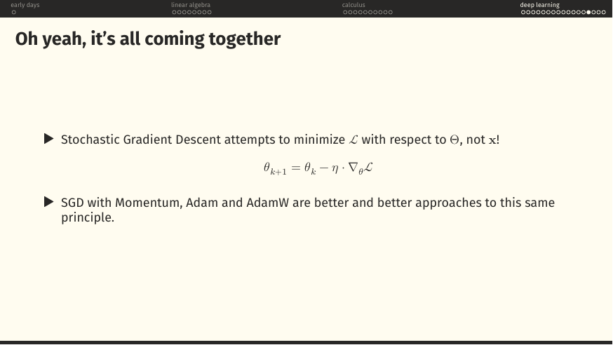
Everything from §3 crystallises into one line:

θ_{k + 1} = θ_{k} - η \cdot \nabla_{θ} L

Note the subscript: the gradient is with respect to $θ$ , not $x$ . Data is fixed; parameters are what we tune. The "S" in SGD is stochastic, we approximate the full gradient by averaging over a random mini-batch of examples at each step, which is faster and, surprisingly, often finds better minima than the exact full-batch version.

Why the family grew

Plain SGD is fine but sensitive to the learning rate and slow in valleys where the loss curves gently along one direction and steeply along another. Momentum adds inertia so you barrel through shallow directions. Adam and AdamW track per-parameter statistics of the gradient's mean and variance and adapt the step size accordingly, think of it as approximating the diagonal of the Hessian on the cheap. All of them are trying to buy Newton-Raphson-style curvature information without paying the Newton-Raphson-style price.

Page 75 / 82

$Newton-Schulz has also been back in the spotlight because of the Muon optimizer.$

page 75 · Newton-Schulz returns

Page 76 / 82

$Algorithm 2 Muon: init B_0=0; for t=1,…: G_t ← ∇_θ L_t(θ_{t-1}); B_t ← μ B_{t-1} + G_t; O_t ← NewtonSchulz5(B_t); θ_t ← θ_{t-1} − η O_t.$

page 76 · the Muon algorithm

What this build shows

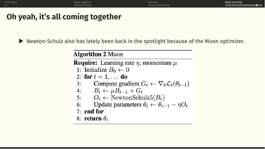
The payoff for the six-page teaser on pages 38-43. The Muon optimizer, in five lines:

Compute the usual gradient $G_{t}$ .
Maintain a momentum buffer $B_{t} = μ B_{t - 1} + G_{t}$ .
Run a Newton-Schulz iteration on $B_{t}$ to orthogonalise it, pushing all its singular values to 1.
Take the resulting matrix $O_{t}$ as the actual update direction.
Update $θ_{t} = θ_{t - 1} - η O_{t}$ .

✦ the aha

Muon literally uses the fact from §2 that any matrix factors as $U Σ V^{T}$ , plus the fact from §3 that odd polynomials commute with this factorisation, to produce an update that is closer to an orthogonal matrix than plain-gradient methods would give. Every idea in this five-line algorithm was introduced earlier in the tutorial. That is the whole point of ordering the material this way.

"Pulling up to the function, the function is English"

Page 77 / 82

$Modern NLP methods treat language as a function: input a tokenised, embedded prompt; output the next token. This is autoregressive LM.$

page 77 · language as a function

Page 78 / 82

$But aren't we approximating functions over Euclidean spaces?$

page 78 · but Euclidean, though?

What this build shows

The moment the tutorial finally says the word "language". Everything we have built, parametrised functions, cross-entropy loss, gradient descent, is deployed on the problem of predicting the next token given a prompt. That prediction problem, chained one token at a time, is autoregressive language modelling. Every LLM you have used is this.

Page 78 raises the obvious objection: our machinery approximates functions on $ℝ^{n}$ . Words are discrete. What gives?

"Sike! It's maths all the way down"

Page 79 / 82

$Outputting embeddings and discretising to the vocabulary is quite weak.$

page 79 · embeddings, discretised, weak

Page 80 / 82

$Instead the output can be a |V|-dimensional vector whose entries are probabilities over the vocabulary — must sum to 1.$

page 80 · probability vector over V

Page 81 / 82

$Softmax: softmax(x)_i = e^{-x_i} / Σ_j e^{-x_j}. Applied as the last-layer activation, it forces outputs to be a valid probability distribution.$

page 81 · softmax

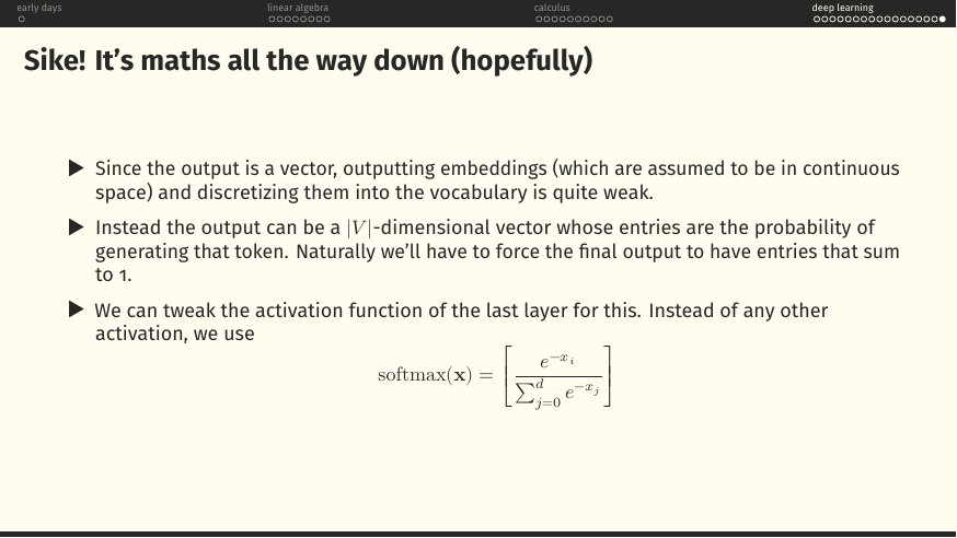
What this build shows

The resolution to page 78's objection. Instead of the network outputting a discrete token (which breaks differentiability), we have it output a $| V |$ -dimensional vector, one number per token in the vocabulary, that we interpret as a probability distribution over what comes next. Sample from it, or just take the arg-max, whenever you actually need a token.

Enforcing the "probability" part

The output vector has to have non-negative entries that sum to 1. The softmax function is the standard way to enforce both:

softmax (x)_{i} = \frac{e^{x_{i}}}{\sum_{j = 1}^{| V |} e^{x_{j}}}

Exponentiate everything to force positivity; divide by the total to force normalisation. Combined with cross-entropy loss (page 62), this is the entire output stage of essentially every language model built in the last decade.

→ where this goes

The very first thing the next tutorial (Matrices → Transformers) does is build the middle layers, attention, MLP blocks, layer norm, that sit between the input embedding and the softmax we just introduced. If this page makes sense, you have all the pre-requisite machinery to follow that next tutorial without pausing.

Page 82 / 82

$Fin.$

page 82 · fin

Fin. Eighty-two pages, four sections, one loop closed. You started with the definition of a vector space; you ended with the softmax layer of a language model. Every idea in between was in service of that trip, and every idea in the rest of the course either uses or extends what this tutorial set up.